What is “naive” in the Naive Bayes Classifier?
The Naive Bayes Classifier is called ‘naive’ because it assumes that each feature is independent of the others. It also assumes that all features are equally important and that they contribute the same to the probability of a given outcome. This seems ‘naive’ because it may not hold true in all cases.
As a specific example, let’s say you are using Naive Bayes Classifier to classify emails as spam or not (based on the words used in the email). The classifier may then classify an email as spam if it finds words such as “discount” or “buy”, and as not spam if it finds words such as “hello” and “thank you”. Since it treats a word as independent it does not take into consideration the context. That means that if someone you trust wants to make you aware of an offer, it could be marked as spam!
What are the differences between Principal Component Analysis (PCA), Singular Value Decomposition (SVD) and Linear Discriminant Analysis (LDA)?
They are all popular linear dimensionality reduction techniques, but they differ in their approach and objectives.
- PCA is a technique that aims to reduce the dimensionality of the data by identifying the most important features that explain the variance in the data. It finds a new set of orthogonal variables (called principal components) that capture the maximum amount of variance in the original data, while minimizing the loss of information.
- SVD is a matrix factorization technique that decomposes a matrix into its singular values and singular vectors. It is used to compress the data, remove noise, and identify patterns in the data. SVD is often used as a pre-processing step for other machine learning algorithms.
- LDA, on the other hand, is a supervised dimensionality reduction technique that aims to find the linear combination of features that best separates different classes in the data. It projects the data onto a lower-dimensional space while preserving class separability.
In summary, PCA and SVD are unsupervised dimensionality reduction techniques that aim to find the most important features that capture the variance in the data or identify patterns, while LDA is a supervised technique that aims to find the features that best separate the classes in the data. Each technique has its own strengths and weaknesses, and the choice of technique depends on the specific objective of the analysis.
What are the differences between multiple regression and multivariate regression?
- Multiple regression involves predicting a single dependent variable using multiple independent variables. It focuses on understanding the relationship between the dependent variable and the independent variables.
- Multivariate regression, on the other hand, predicts multiple dependent variables simultaneously, considering their interdependencies. It is used when there are multiple outcome variables and a larger number of independent variables.
In summary, multiple regression deals with a single dependent variable, while multivariate regression deals with multiple dependent variables simultaneously, accounting for their interrelationships.
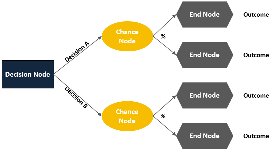
Explain the three types of nodes in decision tree models.
- Decision or choice nodes: represent points in the model where decisions need to be made. These nodes typically arise when there are multiple alternatives or paths to choose from, and the decision-maker must select one option.
- Chance nodes: denote probability nodes. They represent situations or events that are influenced by uncertain or random factors. At chance nodes, probabilities are assigned to various outcomes, reflecting the likelihood of each outcome occurring. This allows for the consideration of uncertainty in decision-making.
- End or outcome nodes: indicate the final outcomes or consequences of a decision or a sequence of events. These nodes represent the end points of the decision-making process, where no further choices or probabilities exist. The end nodes often correspond to specific outcomes or states of the system being modeled.
What is the difference between parametric and non-parametric models in time series forecasting? When would you choose one over the other?
Parametric models assume a specific distribution or functional form for the data, while non-parametric models make fewer assumptions and are more flexible.
Parametric models, such as ARIMA, AR, MA, and exponential smoothing models, are suitable when the data follows a known distribution or has clear patterns, and when interpretability is important.
Non-parametric models, like decision trees, random forests, SVM, and neural networks, are chosen when the data generating process is unknown, exhibits nonlinear relationships, or requires flexibility over interpretability.
The choice depends on the dataset’s characteristics and forecasting goals, and sometimes a hybrid approach combining both models can be effective.
What is The Kernel Trick used in Support Vector Machines?
In Support Vector Machines (SVM), the kernel trick is a clever mathematical technique that allows us to perform complex calculations in a higher-dimensional feature space without explicitly transforming the original data into that space. It is a way to efficiently handle non-linear relationships between data points.
To understand the kernel trick, let’s consider a simple example. Imagine we have a dataset with two classes of points that are not linearly separable in a two-dimensional space. The kernel trick allows us to find a decision boundary, or hyperplane, that can effectively separate these classes by projecting the data points into a higher-dimensional space where they become linearly separable.
Instead of explicitly transforming the data into this higher-dimensional space, which can be computationally expensive or even impossible in some cases, the kernel trick enables us to calculate the inner product between pairs of data points in the higher-dimensional space without actually carrying out the transformation. This is done by defining a kernel function, which computes the similarity or distance between two points in the original feature space.
By using different kernel functions, such as the linear, polynomial, or radial basis function (RBF) kernels, SVM can effectively capture complex relationships between data points. The kernel trick allows SVM to operate efficiently in these high-dimensional spaces, making it a powerful tool for solving both linear and non-linear classification problems.