Part I: Accuracy and Confusion Matrix

There are many different Machine Learning problems, and even within them, there are several ways the objective of the project and the data we have can affect how we assess our model’s performance.

We will start with the evaluation metrics used in classification models.

There are three main types of classification problems:

• Binary classification: there are two classes, generally one positive and one negative. For example, if a patient has a particular disease or not.
• Multi-class classification: it is a generalization of the binary classification problem, with the dataset having more than two classes. For instance, sentiment analysis: happy, sad, worried, surprised…
• Multi-label classification: each sample can have more than one label. For example, detection of animals within a picture, there can be only a dog, but also there can be both a dog and a cat in the same picture.

Depending on the characteristics of our problem we will need to select an adequate metric to assess the performance of the model.

For the sake of simplicity, we will explain the different metrics using a binary classification problem. However, the methods explained for this particular case can then be generalized to the multi-class scenario.

Classification accuracy

The classification accuracy is defined as the quotient between the number of correct predictions and the total number of predictions.

$$ \text{Accuracy} = \frac{\text{Correct predictions}}{\text{Total predictions}} $$

Its complement metric is the classification error, defined as the number of wrong predictions divided by the total number of predictions.

$$ \text{Error} = \frac{\text{Wrong predictions}}{\text{Total predictions}} $$

These metrics are the simplest to interpret and understand, however, they only work as long as we have a balanced dataset and we do not have a preference or special interest in predicting any of the classes.

Confusion matrix

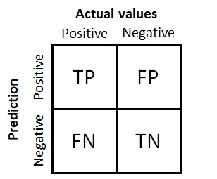
A confusion matrix represents counts for predicted and actual values. It helps us understand how many of the samples are correctly or incorrectly classified in each one of the classes.

Confusion matrix for a binary classification problem.

There are four quadrants in the matrix:

• True Positives (TP): number of positive or relevant samples that were correctly predicted as such.
• True Negatives (TN): number of negative samples that were correctly predicted as negative.
• False Positives (FP): number of positive samples that were incorrectly predicted as negative. This is the so-called type I error in statistics, referring to the wrong rejection of the null hypothesis.
• False Negatives (FN): number of negative samples that were incorrectly predicted as positive. This is the so-called type II error in statistics, referring to the wrong failure to reject the null hypothesis.

In general terms, the purpose of any model is to maximize the number of TP and TN, and therefore minimize the FP and FN.

To find out the total number of samples or predictions, the values in the four quadrants must be added up:

$$ \text{Total predictions} = TP + TN + FN + FP $$

The confusion matrix will help us define more complex metrics, as well as redefine the previous ones:

$$ \text{Accuracy} = \frac{TP + TN}{TP + TN + FN + FP} $$

$$ \text{Error} = \frac{FP + FN}{TP + TN + FN + FP} $$

The rest of the evaluation metrics used in classification problems will be explained in the next article.