Normal distribution: scaling and missing values

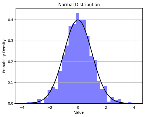
A normal distribution, also known as a Gaussian distribution, is a continuous probability distribution that is symmetrically shaped like a bell curve.

The following set of statistical properties characterizes it:

1. Symmetry: The distribution is symmetric around its mean, which is also the median and mode of the distribution. This means that the left and right sides of the distribution are mirror images of each other.
2. Bell-shaped curve: The graph of a normal distribution is bell-shaped, with the highest point at the mean. As you move away from the mean in either direction, the probability of observing values decreases.
3. Mean, Median, and Mode: In a normal distribution, the mean, median, and mode are all equal and located at the centre of the distribution.
4. Standard Deviation: The spread or dispersion of the data is measured by the standard deviation. The standard deviation determines the width of the bell curve. A larger standard deviation results in a wider and flatter curve, while a smaller one results in a narrower and taller curve.
5. Empirical Rule (68-95-99.7 Rule): In a normal distribution, approximately 68% of the data falls within one standard deviation of the mean, about 95% falls within two standard deviations, and around 99.7% falls within three standard deviations.

The normal distribution is a fundamental concept in statistics and probability theory, and it is widely used in various fields to model and analyze random variables. Many natural phenomena and measurements, such as height, IQ scores, and errors in measurements, often exhibit a normal distribution. The mathematical equation for the probability density function (PDF) of a normal distribution is given by the famous bell-shaped curve formula:

$$ f(x) = \frac{1}{\sigma \sqrt{2\pi}} \exp\left(-\frac{1}{2}\left(\frac{x – \mu}{\sigma}\right)^2\right) $$

where:

• $ \mu $ is the mean,
• $ \sigma $ is the standard deviation,
• $ \pi $ is a mathematical constant (approximately 3.14159),
• $ e $ is the base of the natural logarithm (approximately 2.71828), and
• $ x $ is the variable of the distribution.

How to treat normally distributed features?

Depending on the distribution of your data you will need to consider different approaches. In this article we are dealing with the Gaussian or Normal distribution, the most typical one in Data Science.

In addition to all the visualization and data understanding steps, we can differentiate three typical operations that we could do to features that specifically follow a normal distribution during the Exploratory Data Analysis (EDA) and Data Cleaning/Processing stages. These are scaling, detecting and handling outliers and addressing missing values.

Scaling

When a feature is normally distributed, scaling is important to ensure that the feature values have a standard scale, especially for algorithms that are sensitive to the scale of the data. Standard scaling (subtracting the mean and dividing by the standard deviation) ensures that the feature has a mean of 0 and a standard deviation of 1.

from sklearn.preprocessing import StandardScaler 

# Instantiate StandardScaler 
scaler = StandardScaler() 

# Fit and transform the data 
scaled_data = scaler.fit_transform(df) 

# Create a new DataFrame with the scaled data 
scaled_df = pd.DataFrame(scaled_data, columns=df.columns) 

Missing values

Missing values refer to the absence of certain data points or values in a dataset and they can be a problem for several reasons:

1. Biased Analysis: If the missing values are not handled properly, it can lead to biased analysis and inaccurate model predictions.
2. Reduced Sample Size: Missing values reduce the effective sample size, which can impact the statistical power of the analysis and the performance of machine learning models.
3. Algorithm Sensitivity: Many machine learning algorithms cannot handle missing values directly. They may either produce an error or give biased results if missing values are not addressed.

To identify missing values in a dataset, you can visualize each feature using graphs such as histograms, bar charts, or heatmaps. Here you can see an example of a heatmap using the python library seaborn:

import matplotlib.pyplot as plt
import seaborn as sns

# Create a heatmap of missing values
sns.heatmap(df.isnull(), cbar=False, cmap='viridis')

# Show the plot
plt.show()

Also, you could simply use the following code:

# Check for missing values in each column
missing_values = df.isnull().sum()

# Display the count of missing values for each column
print(missing_values)

Once identified, the majority of algorithms require you to address them. Since we are dealing in this article with normally distributed features, we will consider the following two strategies. This can change if you have sufficient domain knowledge and are aware of other more suitable strategies.

Mean Imputation

Since the data is normally distributed, using the mean to fill in missing values is a reasonable approach. This method preserves the mean of the distribution, making it a suitable choice for data with a normal distribution.

mean_value = df['feature'].mean()
df['feature_mean_imputed'] = df['feature'].fillna(mean_value)

Median Imputation

Although the mean is generally preferred for normally distributed data, median imputation can be used as a robust alternative, especially if there are outliers. The median is less sensitive to outliers and can be a better measure of central tendency in such cases.

median_value = df['feature'].median()
df['feature_median_imputed'] = df['feature'].fillna(median_value)

In the next article, we will proceed with the identification and handling of outliers in normally distributed features.