Clean your Time Series data III: Outliers removal

In the first two parts of this series, we discussed the importance of cleaning time series data and covered techniques for handling missing data and dealing with duplicate values. In this third, we’ll delve into an important aspect of cleaning time series data: outlier removal.

Remove outliers

Outliers are data points that deviate significantly from the rest of the data. They can be caused by measurement errors, data entry errors, or even natural variations in the data. Outliers can have a significant impact on the analysis of time series data, as they can skew statistical measures such as the mean and standard deviation, and can even lead to incorrect conclusions.

Outliers identification

Visual inspection

We should always start by visualizing our data. This is an essential first step in identifying outliers. By creating a time series plot, we can examine the patterns and trends of the data, and visually inspect for any abnormal spikes or dips. Outliers can appear as data points that are significantly distant from the rest of the data, and these can be identified by examining the plot for any unusual or unexpected fluctuations. Therefore, visual inspection of the time series plot can be an effective and intuitive way to detect outliers in time series data.

Box-plot

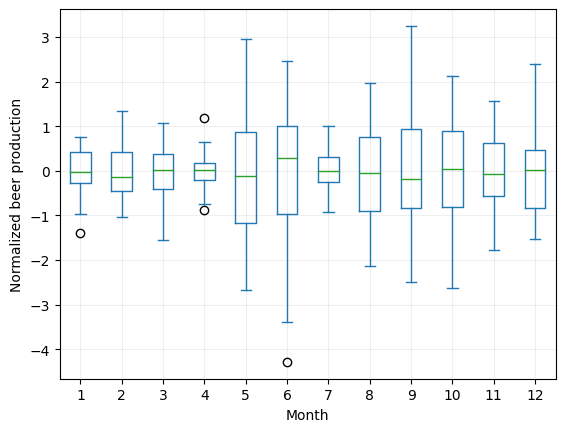
However, we need a more robust technique to clearly identify them. One way is to use a box plot. A box plot shows the distribution of the data and identifies any outliers as points that fall outside the “whiskers” of the plot.

In our case, we have monthly data, so it would be better if we group them by month to find the outliers:

 # Group by month
df_beer.set_index(df_beer.index.month, append=True).Production.unstack().plot.box()
plt.xlabel('Month')
plt.ylabel('Normalized beer production')
plt.grid(which='both', alpha=0.2)
plt.show()

Interquartile range test

We have identified four outliers in our dataset. To identify these outliers, we used the interquartile range (IQR) test.

The interquartile range test is a statistical method used to identify potential outliers in a dataset. It involves calculating the difference between the first quartile (Q1) and the third quartile (Q3) of the data distribution, which represents the middle 50% of the data.

The IQR is then multiplied by a constant factor, typically 1.5, to define the lower and upper limits of the expected range of data values. Data points that fall outside of this expected range are considered potential outliers.

$ [( \text{Q1}-1.5 \text{IQR}), ( \text{Q3}+1.5 \text{IQR})] $

To apply the interquartile test, we first sort the data in ascending order and then calculate the values of Q1 and Q3. These can be calculated as the median of the lower half of the data and the median of the upper half of the data, respectively. The IQR is then calculated as Q3 minus Q1.

The lower limit of the expected range is defined as Q1 minus 1.5 times the IQR, and the upper limit is defined as Q3 plus 1.5 times the IQR. Any data points that fall outside of these limits are considered potential outliers and should be further examined and verified.

One advantage of the interquartile test is that it is less sensitive to extreme values than the next test, the Z-score test, which makes it more suitable for datasets with skewed or non-normal distributions. However, it may not be as effective in detecting outliers in small sample sizes or datasets with multiple modes.

# Remove outliers according to month
 
abnormal_values_dates = []

for month in range(13):

    # Group values by month
    df_month = df_beer[df_beer.index.month == month]
    
    # Calculate Q1, Q3 and interquartile range
    q1 = df_month.Production.quantile(0.25)
    q3 = df_month.Production.quantile(0.75)
    iqr = q3 - q1
    
    # Find anomalies
    abnormal_dates = df_month[(df_month.Production < q1 - 1.5 * iqr) \
                         | (df_month.Production > q3 + 1.5 * iqr)].index
    
    # Add anomalies to list
    if not abnormal_dates.empty:
      abnormal_values_dates = abnormal_values_dates + list(abnormal_dates)

Z-score test

The Z-score test is a commonly used statistical method for identifying outliers in time series data. One approach is to use the normalized data and consider any data points above or below a certain threshold as outliers. Typically, the threshold is set at 3 and -3 standard deviations from the mean, but this can vary depending on the specific case.

When working with time series data, it’s common to calculate the Z-score using a rolling window approach. This means that we only consider the data points within a specified window of time, typically the past few days, months or years, to calculate the mean and standard deviation. By using a rolling window, we can ensure that our analysis is more focused on recent trends and patterns in the data.

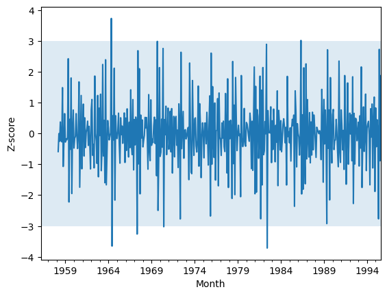
While we have already ensured that our time series data is stationary, we can still use the Z-score test with a 24-month rolling window for a more complete analysis. By doing so, we can identify any data points that fall outside of the expected range and consider them as potential outliers that require further investigation.

# Define the z-score function
def zscore(x, window):
    r = x.rolling(window=window)
    m = r.mean().shift(1)
    s = r.std(ddof=0).shift(1)
    z = (x-m)/s
    return z
    
# Calculate zscore with a rolling window and get abnormal values
window_size = 24 
df_zscore = zscore(df_beer, window_size)

# Apply a threshold for the z-score
threshold = 3
abnormal_values_dates = df_zscore[abs(df_zscore.Production) > threshold ].index

Anything outside the blue-shaded area can be considered an anomaly according to our specified threshold.

Outliers removal

Once outliers have been identified, they can be removed from the data set. However, it’s important to be careful when removing outliers, as they can contain important information about the data. If an outlier is caused by a measurement error, for example, it may be appropriate to remove it. But if an outlier is caused by natural variation in the data, removing it could lead to incorrect conclusions.

We will set them to NaN so we can deal with them later:

# Set anomalies to NaN
df_beer.loc[abnormal_values_dates, 'Production'] = np.nan

You could now proceed with several options. One of them is calculating the average production per month and imputing these values:

# Calculate the average production per month
monthly_avg = df_beer.groupby(df_beer.index.month).mean()

# Impute these values
for month in monthly_avg.index:
    df_beer.loc[df_beer.index.month == month, 'Production'] = \
        df_beer.loc[df_beer.index.month == month, 'Production'].fillna(
            monthly_avg.loc[month, 'Production'])

Alternatively, you could consider simpler imputation methods, such as linear interpolation:

# Interpolate
df_beer = df_beer.interpolate()

It all depends on your particular case. Try different strategies and assess the best case for you.

In conclusion, removing outliers from time series data is an essential step in ensuring accurate and reliable analysis. Outliers can significantly affect the results of statistical analyses, and thus, it is crucial to identify and remove them before drawing any conclusions. We have discussed several techniques for detecting and removing outliers, including visual inspection, the box-plot method, the interquartile range test and the Z-score test. Each method has its strengths and weaknesses, and the most suitable approach will depend on the nature of the data and the research question being addressed. However, it is essential to remember that the removal of outliers should always be done with caution and should be based on a thorough understanding of the data and its context. By taking these steps, we can ensure that our analysis is accurate, reliable, and free from the influence of outliers.

See all the parts of the data cleaning series:

1. Missing values and detrending
2. Remove seasonality and normalize data
3. Outliers removal
4. Data Smoothing

We are now a step closer to being able to start building our model!

You can access the notebook in our repository:

GitHub – MLPills/remove-outliers: A Jupyter Notebook that covers the basics of removing outliers

A Jupyter Notebook that covers the basics of removing outliers – GitHub – MLPills/remove-outliers: A Jupyter Notebook that covers the basics of removing outliers

github.com

To run it right now click on the icon below:

We will see in the next article how we can smooth our data!