This previous article introduced the importance of correctly handling dates when working with time series data. In Python, there are multiple use cases and tools that must be known. This article is a continuation of the previous one, and we will explore more advanced techniques and tools to manipulate dates and datetime-related features.
Converting Strings to Datetime Objects
In Python, you can convert a string representing a date or time into a datetime object using the strptime() function from the datetime module. This function parses a string representing a date and/or time according to a given format and returns a datetime object.
from datetime import datetime

date_string = "2024-02-02"
date = datetime.strptime(date_string, "%Y-%m-%d")
datetime.datetime(2024, 2, 2, 0, 0)
In the above code:
date_stringrepresents the date in the format'YYYY-MM-DD'.%Y,%m, and%dare format codes that represent year, month, and day respectively. These codes are used to specify the format of the input string.
Converting Datetime to Strings
Conversely, you can convert a datetime object to a string using the strftime() function from the datetime module. This function formats a datetime object into a string according to the specified format.
from datetime import datetime

date = datetime.now()
date_string = date.strftime("%Y-%m-%d")
'2024-02-09'
In this code:
dateis adatetimeobject representing the current date and time.%Y-%m-%dis the format string used instrftime().%Yrepresents the year,%mrepresents the month, and%drepresents the day.
Both of these conversions are commonly used when working with dates and times in Python, especially when dealing with input/output operations or when manipulating date/time data.
Below you can check the most common directives for formatting datetime data. You can find the rest of them here.
| Directive | Meaning | Example |
| %a | Abbreviated weekday name. | Sun, Mon, … |
| %A | Full weekday name. | Sunday, Monday, … |
| %w | Weekday as a decimal number. | 0, 1, …, 6 |
| %d | Day of the month as a zero-padded decimal. | 01, 02, …, 31 |
| %b | Abbreviated month name. | Jan, Feb, …, Dec |
| %B | Full month name. | January, February, … |
| %m | Month as a zero-padded decimal number. | 01, 02, …, 12 |
| %y | Year without century as a zero-padded decimal number. | 00, 01, …, 99 |
| %Y | Year with century as a decimal number. | 2013, 2019 etc. |
| %H | Hour (24-hour clock) as a zero-padded decimal number. | 00, 01, …, 23 |
| %I | Hour (12-hour clock) as a zero-padded decimal number. | 01, 02, …, 12 |
| %p | AM or PM indicator. | AM, PM |
| %M | Minute as a zero-padded decimal number. | 00, 01, …, 59 |
| %S | Second as a zero-padded decimal number. | 00, 01, …, 59 |
| %z | UTC offset in the form +HHMM or -HHMM. | +0000, -0400, +1030 |
| %Z | Time zone name. | UTC, GMT |
Shifting and Lagging
Shifting or lagging time series data is essential in certain scenarios, especially in feature engineering, where incorporating previous values or changes as features for your model can significantly enhance predictive capabilities.
By shifting the time series data, we can create lag features that capture historical patterns and trends, providing valuable context for predictive models. This approach enables the model to learn from past behavior and make more accurate forecasts, improving overall performance and decision-making.
# Shift forward
df['forward'] = df['value'].shift(1)

# Shift backward
df['backward'] = df['value'].shift(-1)
This is how the outcome looks when you plot it:
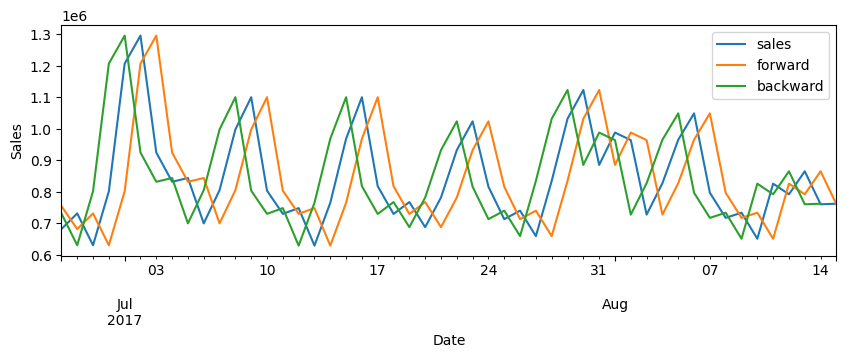
When performing shifting or lagging operations on time series data, it’s important to note that NaN (Not a Number) values will appear. These NaNs occur because shifting moves the data points forward or backward, leaving gaps at the beginning or end of the series where the shifted values are not defined. Handling these NaNs appropriately is crucial, as they can affect subsequent analysis or modeling processes. You can learn how to handle them below.
Differencing
Time series differencing involves computing the difference between consecutive observations in a time series. This technique is crucial, particularly in feature engineering, as it enables the creation of new features that capture changes or trends over time.
By differencing the time series data, we can remove trends and seasonality, making the series stationary and facilitating the modeling of underlying patterns. Incorporating differenced features into predictive models allows us to capture short-term fluctuations and changes in the data, improving their ability to forecast future values accurately.
 # Difference with the previous value
 df['diff'] = df['value'].diff()
When we perform the difference, we can see that the new feature is the difference between the current observation and the previous one:
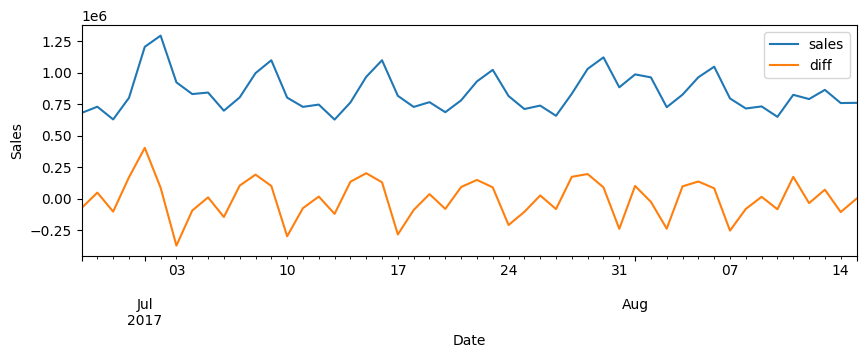
When differencing time series data NaN values will also arise. These NaNs can occur due to the absence of a previous observation to compute the difference with the first data point or when differencing results in missing values. Proper handling of these NaNs is vital to ensure accurate analysis and modeling, as they can impact subsequent calculations and interpretations of the data. You can learn how to handle this in the next section.
Overall, differencing time series data plays a fundamental role in feature engineering, enhancing the predictive capabilities of models by capturing temporal dynamics and trends effectively. This will allow you to account for the sequential aspect of time series data or to determine if there have been increases or decreases in the values indicating trends.
Missing Dates
Real-world datasets often come with missing dates. To address missing dates in a DataFrame, one effective method is utilizing the asfreq function in pandas. This function allows you to conform a DataFrame to a specified frequency, adding missing dates as needed. Importantly, the asfreq function operates on the DataFrame index, ensuring that missing dates are correctly aligned and added where necessary.
This will generate missing values, to handle this you have multiple approaches to employ:
A common approach is forward filling, where the last valid observation is propagated forward. This method is useful for scenarios such as analyzing daily stock prices, where missing dates occur due to holidays or weekends, ensuring that the most recent available data is used for analysis without any gaps.
Alternatively, backward filling utilizes the next valid observation to fill gaps. This approach might be employed in analyzing monthly sales data, where missing dates might occur due to incomplete records or delays in reporting, ensuring that future data points are not used prematurely, and gaps are filled with the most recent available information.
df = df.asfreq('D')  # ensure daily data with no missing dates

# Apply one of these filling methods
df = df.fillna(method='ffill')  # forward fill
df = df.fillna(method='bfill')  # backward fill
In this snippet first, we make sure there are no missing dates, by using asfreq. Then we apply one of the mentioned methods. These two methods are widely used. However, you need to know when to use each one.
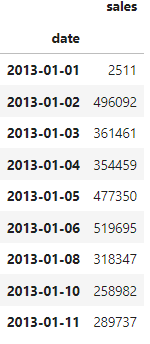
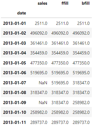
Let’s show an example. We’ll start from this dataframe, which has 2 dates missing (7th and 9th of January):
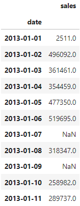
After using asfreq we get the following, with 2 missing values as expected:
When we apply the forward and backward fill we obtain the following:
There are also other common methods such as:
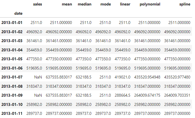
Mean/Median/Mode Imputation: Missing values are filled with the mean, median, or mode of the non-missing values in the same column. This method is straightforward but may not capture the true distribution of the data.
# Fill missing values with mean
df_mean_filled = df.fillna(df.mean())

# Fill missing values with median
df_median_filled = df.fillna(df.median())

# Fill missing values with mode (most frequent value)
df_mode_filled = df.fillna(df_miss['sales'].mode()[0])
The interpolation method estimates missing values based on the surrounding observed values. Common interpolation techniques include linear interpolation, polynomial interpolation, and spline interpolation.
# Interpolate missing values using linear interpolation
df_linear_interpolated = df.interpolate(method='linear')

# Interpolate missing values using polynomial interpolation (order 2)
df_polynomial_interpolated = df.interpolate(method='polynomial', order=2)

# Interpolate missing values using spline interpolation
df_spline_interpolated = df.interpolate(method='spline', order=2)
And this is the outcome of the last methods:
There is still a lot more to cover, like reindexing, dealing with time zones… Don’t miss the next article. Also, don’t forget to check the previous one.


0 Comments