Time Series Forecasting with STL

STL stands for “Seasonal and Trend decomposition using LOESS”. It is a versatile and robust method for decomposing time series. This method decomposes a time series into its three main components:

1. Trend: The underlying trend of the data.
2. Seasonal: Seasonal effects.
3. Residual: The remainder after accounting for the trend and seasonal components.

Classical decomposition methods vs. STL

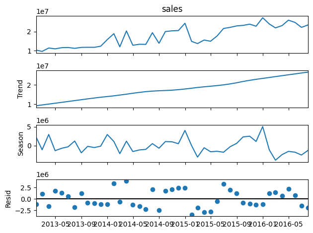
Before carrying on with STL, let’s introduce traditional methods. Here you have an example of the Seasonal Decompose method to extract the three components, which was shown in a previous article:

This decomposition method, Seasonal Decompose, uses Moving Averages to split the time series data into trend, seasonality, and noise. Then the trend is extrapolated on both extremes. It is best for datasets with clear and consistent seasonal patterns. It assumes that the seasonal component repeats identically over time. However, Seasonal Decompose often struggles with edge data points due to its reliance on moving averages, which can result in missing information at the beginning and end of the series. Also, it is not capable of extracting changing seasonality and trends.

STL, on the other hand, offers a more advanced approach. Utilizing LOESS (Locally Estimated Scatterplot Smoothing), it flexibly decomposes a time series, adapting to changing trends and seasonality. This makes it suitable for more complex datasets. It is particularly valuable when dealing with non-linear trends and evolving seasonal patterns. Although more computationally demanding, its adaptability makes it a preferred choice for detailed and dynamic time series analysis.

Inputs

The key inputs into STL are:

• Length of the Seasonal Smoother: This is the window size used to estimate the seasonal component in the STL decomposition. It must be an odd number to ensure symmetry around the central point. The larger the window size, the smoother the estimated seasonal component will be. If the window size is too small, the seasonal component may capture some of the trend, and if it’s too large, some of the seasonality may be missed.
• Length of the Trend Smoother: This is the window size used to estimate the trend component in the STL decomposition. It must be an odd number and larger than the length of the seasonal smoother. This is to ensure that the trend component does not capture any of the seasonal fluctuations. Usually, it’s around 150% of the length of the seasonal smoother, but this can be adjusted based on the specific characteristics of your time series.
• Length of the Low-Pass Estimation Window: This is the window size used in the low-pass filter, which is a part of the STL decomposition process. The low-pass filter is used to remove the high-frequency fluctuations (noise) from the time series. The length of the low-pass estimation window is usually the smallest odd number larger than the periodicity of the data. This is to ensure that the low-pass filter does not remove any of the seasonal fluctuations.

Advantages and Disadvantages

STL has several advantages over classical decomposition methods:

1. Versatility: STL can handle any type of seasonality, not just monthly or quarterly data. This makes it applicable to a wide range of time series data.
2. Robustness: STL is robust to outliers. This means that occasional unusual observations will not affect the estimates of the trend-cycle and seasonal components.
3. Flexibility: The seasonal component is allowed to change over time, and the rate of change can be controlled by the user. This allows STL to adapt to time series data where the seasonality is not constant.
4. Control over Smoothness: The smoothness of the trend-cycle can be controlled by the user. This allows the user to tailor the decomposition to the specific characteristics of their data.
5. Decomposition into Components: STL decomposes a time series into three components: trend, seasonal, and residual. This can provide valuable insights into the underlying patterns in the data.

However, it also has some disadvantages:

1. Additive Decomposition Only: STL only provides facilities for additive decompositions. It does not support multiplicative decompositions directly, although you can transform your series (e.g., by taking the log) before applying STL if a multiplicative decomposition is needed.
2. No Automatic Handling of Trading Day or Calendar Variation: STL does not automatically handle variations that occur due to the trading day or calendar effects. These would need to be handled separately.
3. Requires Specification of Parameters: The user needs to specify several parameters. Incorrect specification of these parameters can lead to poor decomposition results.
4. No Forecasting Capability: STL is a tool for decomposition, not forecasting. While the trend and seasonality extracted from STL can be used to build a forecast model, STL itself does not provide any forecasting capabilities.
5. Not Suitable for All Time Series: STL assumes that the time series is a combination of seasonality, trend, and residuals. This may not be the case for all time series, especially those with complex structures or non-standard patterns.
6. Sensitive to Outliers: Although STL can be made robust to outliers, extreme values can still impact the trend and seasonality extraction. This is because the LOESS smoother used in STL can be influenced by high leverage points.

STL to forecast Time Series data

To use STL for forecasting time series data, you can follow these general steps:

1. Decompose the Time Series: Use STL to decompose the time series into trend, seasonal, and residual components.
2. Deseasonalize the Time Series: Subtract the seasonal component from the original time series to get a deseasonalized time series.
3. Forecast the Deseasonalized Time Series: Apply a non-seasonal forecasting method (like ARIMA or Exponential Smoothing) to the deseasonalized time series. This will give you a forecast of the trend and residual components.
4. Forecast the Seasonality: For the seasonal component, STL assumes that the future seasonal component will repeat the last observed seasonal cycle. So, if you have monthly data with a yearly cycle, it will take the seasonal component from the last year and repeat it for the forecast period.
5. Reapply the Seasonal Component: Add the “forecasted” seasonal component back into the forecasted deseasonalized data. This step is crucial as it retransforms the forecasted data back into the original measurement scale.

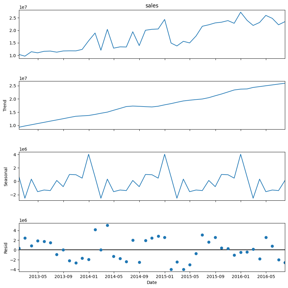
Let’s first see each of the components that STL extracts:

import pandas as pd
import matplotlib.pyplot as plt
from statsmodels.tsa.seasonal import STL

# Import your data
data = pd.read_csv('sales_data.csv').sales

# Decompose the time series with STL (data must be 1D)
stl = STL(data, seasonal=13)
result = stl.fit()

# Plot results
result.plot()
plt.show()

We selected a value for seasonal equal to 13 and the rest of the parameters were left as default. seasonal must be an odd integer and should normally be greater than or equal to 7. A value of 7 or more is suggested to ensure that the seasonal component is sufficiently smoothed and not overly influenced by noise in the data. However, the optimal value can depend on your specific data and the nature of the seasonality. It may require some experimentation and should be guided by the quality of the resulting decomposition and its appropriateness for your specific use case. In our case, since we have a seasonality of 12 (one year with monthly frequency), choosing 13 for the seasonal parameter means that the seasonal component at each point is being smoothed over an entire year (12 months) plus one additional point. This helps to ensure that the seasonal component captures the full cycle of the seasonality.

We can see how in this case, contrary to what happened in the Seasonal Decompose method, the seasonality is not constant (the seasonal period is).

Before proceeding with the steps you would normally take, let’s first introduce a more step-by-step process to understand what is behind this method. We already trained the STL model in the previous code block, let’s now deseasonalize the data and forecast each component (trend and seasonal component) separately.

from statsmodels.tsa.arima.model import ARIMA

# Deseasonalize the time series
deseasonalized = data - result.seasonal

# Fit an ARIMA model - finding the optimal order is another step
model = ARIMA(deseasonalized, order=(1,1,0))
model_fit = model.fit()

# Forecast the next seasonal period
forecast = model_fit.forecast(steps=12)

# Add the seasonal component back in
seasonal_component  = result.seasonal[-12:]
forecast += seasonal_component  

We chose to forecast 12 periods or steps for simplicity, but you could choose the number you prefer. This function could help you work out the seasonal_component forecast depending on the steps you choose:

def forecast_seasonal_component(result, steps, seasonal_period):
    # Repeat the seasonal component
    seasonal_component = np.tile(result.seasonal[-12:], steps // 12)

    # If steps is not a multiple of 12, add the remaining months
    if steps % 12:
        seasonal_component = np.concatenate([seasonal_component, result.seasonal[-12:-12+steps%12]])

    return seasonal_component 

Here, we have assumed an ARIMA order of (1, 1, 0). Ideally, we should determine the optimal order, for instance, by examining the ACF and PACF graphs or employing AutoARIMA. You can find the latter here:

# Import the library
from pmdarima.arima import auto_arima

# Build and fit the AutoARIMA model
model = auto_arima(deseasonalized, seasonal=False, suppress_warnings=True)
model.fit(deseasonalized)

# Check the model summary
model.summary()

Now that we know about the general process, we can show a more compact and straightforward way. The first steps are the same, but the last ones are now automatized. For example, we don’t need to work out the seasonal component, it is automatically handled.

from statsmodels.tsa.forecasting.stl import STLForecast
from statsmodels.tsa.arima.model import ARIMA

# Fit your data and specify the model for the deseasonalized data
stlf = STLForecast(data, ARIMA, model_kwargs={"order": (1, 1, 0)})
model = stlf.fit()

# Forecast data
forecasts = model.forecast(steps=12)

And that’s it! Here is the plot showing training data, testing data and forecasts. In this case, we’ve used a dataset containing store sales:

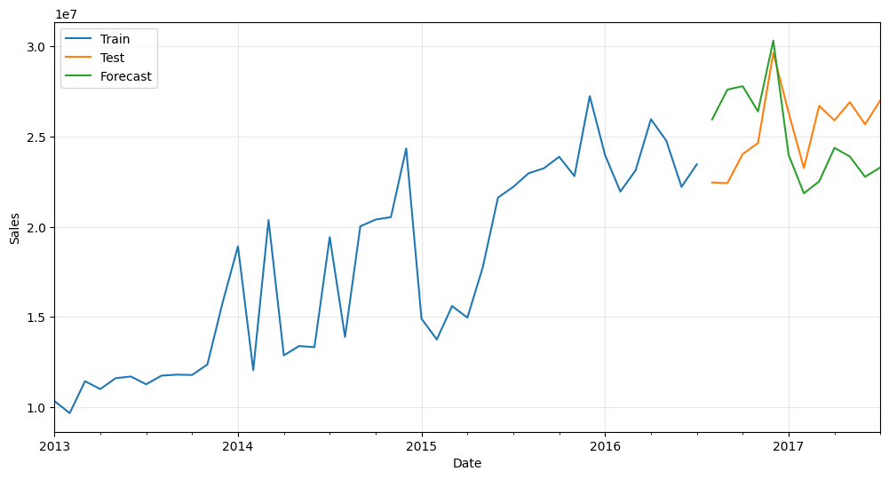
Not too bad for such a simple approach! We could make it slightly more complex, like more robust or see the influence of the different parameters. But that’s for a future article.