We have talked about ARIMA and SARIMA models previously, however, we have never shown a real case step by step.
Let’s first recap, to make sure we know what an ARIMA model is.
ARIMA model
ARIMA (Auto-Regressive Integrated Moving Average) is a popular time series forecasting model that combines autoregressive (AR) and moving average (MA) components with differencing to handle non-stationary data. Let’s have a look at its three components:
- Autoregressive (AR): It models the linear relationship between the current observation and a number
pof lagged observations. It captures the dependency of the current value on its past values. - Moving Average (MA): It models the dependency of the current observation on a number
qof residual errors from previous observations. It captures the short-term shocks or random fluctuations in the data. - Integration (I): It accounts for the differencing required to make the time series stationary. Differencing involves subtracting the previous observation from the current observation to remove trends or seasonality. The order of differencing, denoted by
d, represents the number of times differencing is applied to achieve stationarity.
By combining these three components (AR, I, MA), the ARIMA model is capable of capturing the linear dependencies and trends in time series data. The order of the ARIMA model is typically represented as (p, d, q), where ‘p’ represents the order of the AR component, ‘d’ represents the order of differencing, and ‘q’ represents the order of the MA component.
Stay up-to-date with our latest articles!
Subscribe to our free newsletter by entering your email address below.
SARIMA model
It may be the case that your data has a seasonal component too. This is also something that ARIMA can model. However, we will need to use an extension called SARIMA, which stands for Seasonal ARIMA. This incorporates seasonal components to handle time series data with recurring patterns at fixed intervals, such as daily, weekly, or yearly cycles.
In addition to the autoregressive (AR), moving average (MA), and integration (I) components of ARIMA, SARIMA introduces seasonal AR, seasonal MA, and seasonal I terms to capture the seasonal patterns. The seasonal AR terms represent the relationship between the current observation and its lagged observations at seasonal intervals, while the seasonal MA terms capture the dependence on the lagged residuals at seasonal intervals. The seasonal integration component I accounts for seasonal differencing to remove seasonal trends.
The order of the seasonal ARIMA model is typically denoted as (p, d, q)(P, D, Q, m), where the lowercase parameters refer to the non-seasonal components, and the uppercase parameters represent the seasonal components.
ARIMA and SARIMA models offer a flexible framework for capturing complex patterns and dynamics in time series data and can provide valuable insights for decision-making and future predictions.
Practical case
Let’s see a practical example now. We will try to forecast the maximum monthly temperature in Madrid in 2022.
We need to first import some basic libraries.
import numpy as np
import pandas as pd
import matplotlib.pyplot as plt
import datetime
To get the data we will use the meteostat library:
# Install library
!pip install meteostat

# Import Meteostat library and dependencies
from meteostat import Point, Monthly

# Set time period
start = datetime.datetime(1970, 3, 1)
end = datetime.datetime(2022, 12, 31)

# Create Point for Madrid
location = Point(40.416775, -3.703790, 657)

# Get daily data for March 2023
df_madrid = Monthly(location, start, end)
df_madrid = df_madrid.fetch()
Let’s remove unwanted columns and keep only the maximum temperature.
# Keep only the maximum temperature
df_temp_max = df_madrid[['tmax']]

# Visualize the data
df_temp_max.plot(figsize=(10,5))
plt.grid(alpha=0.5)
plt.xlabel('Date')
plt.ylabel('Maximum temperature')
plt.show()
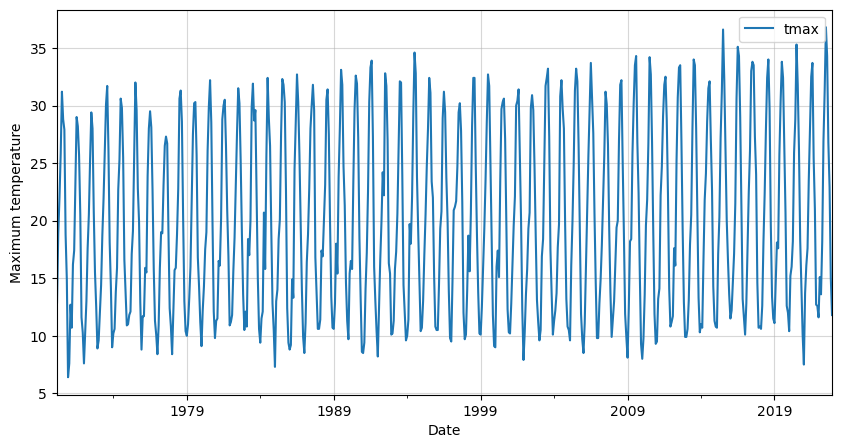
We can clearly see a seasonal pattern in our data. This is to expect as we are dealing with monthly temperatures.
We need to make sure that there are no missing values. If there were, we would need to handle them.
# Check for missing values
df_temp_max.isna().sum()
tmax 0
dtype: int64
Fortunately for us, there are no missing values in our data.
Let’s now proceed to decompose our data, to verify the presence of a seasonal component. We can use the seasonal_decompose function of the statsmodels library.
We will assume a seasonal period of 12 since we have monthly data. Also, there is nothing in the data that makes us suspect a multiplicative model, the variance is not either increasing or decreasing significantly. Therefore, we will use an additive model.
# Import statsmodels library
import statsmodels.api as sm

# Perform seasonal decomposition
decomposition = sm.tsa.seasonal_decompose(df_temp_max,
                                          model='additive',
                                          period=12)

# Extract the decomposed components
trend = decomposition.trend
seasonal = decomposition.seasonal
residual = decomposition.resid

# Plot the decomposed components
decomposition.plot()
plt.show()
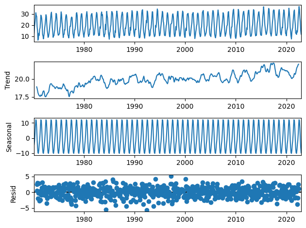
This confirms our suspicion of seasonality in the data. Therefore, we will use a SARIMA model to forecast the future maximum temperatures in Madrid.
Check for stationarity
We could check stationarity, however, this is not necessary as we will use a SARIMA model.
However, it could be useful to estimate the d parameter and speed up the process.
We can use the Augmented Dickey–Fuller test to see whether there is a unit root in our time series data.
from statsmodels.tsa.stattools import adfuller

# Perform Augmented Dickey-Fuller test
result = adfuller(df_temp_max)

# Extract and print the test statistics and p-value
test_statistic = result[0]
p_value = result[1]
print(f"Test Statistic: {test_statistic}")
print(f"P-value: {p_value}")
Test Statistic: -2.971872590243202
P-value: 0.03760595188739091
We got a p-value lower than 0.05, therefore, we can assume that our data is stationary.
Since the p-value is in the limit, let’s also use a Kwiatkowski–Phillips–Schmidt–Shin (KPSS) test to verify our assumption. This test examines the presence of a trend or other forms of non-stationarity.
from statsmodels.tsa.stattools import kpss

# Perform KPSS test
result = kpss(df_temp_max)

# Extract and print the test statistic and p-value
test_statistic = result[0]
p_value = result[1]
print(f"Test Statistic: {test_statistic}")
print(f"P-value: {p_value}")
Test Statistic: 0.23003042556646808
P-value: 0.1
In this case, we are interested in a p-value larger than 0.05. This is because of how the hypotheses are defined. The p-value is larger than 0.05 and therefore it confirms the stationarity of the data.
This is telling us that the d parameter will be 0, or what is the same, that no differencing will be necessary.
For the sake of completeness, we could check the ACF and PACF plots. This can confirm the presence of seasonality and the seasonal period.
from statsmodels.graphics.tsaplots import plot_acf, plot_pacf

# Plot ACF
fig, ax = plt.subplots(figsize=(10, 5))
plot_acf(df_temp_max, ax=ax)
plt.xlabel('Lag')
plt.ylabel('Autocorrelation')
plt.title('Autocorrelation Function (ACF)')
plt.show()

# Plot PACF
fig, ax = plt.subplots(figsize=(10, 5))
plot_pacf(df_temp_max, ax=ax)
plt.xlabel('Lag')
plt.ylabel('Partial Autocorrelation')
plt.title('Partial Autocorrelation Function (PACF)')
plt.show()
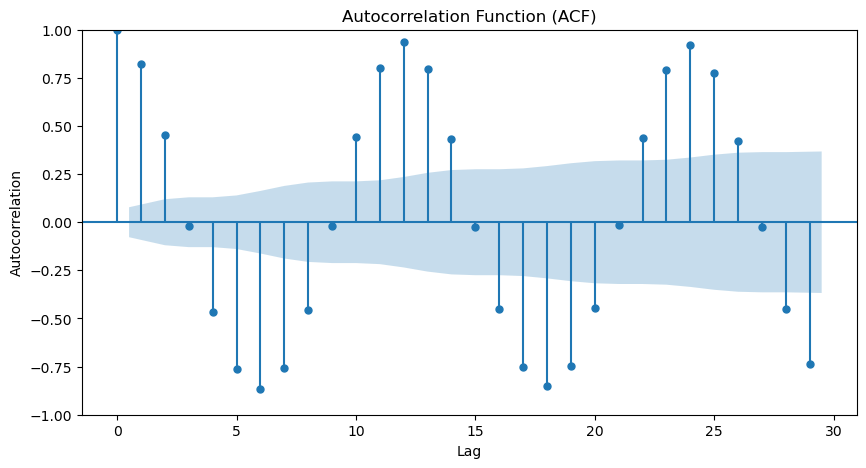
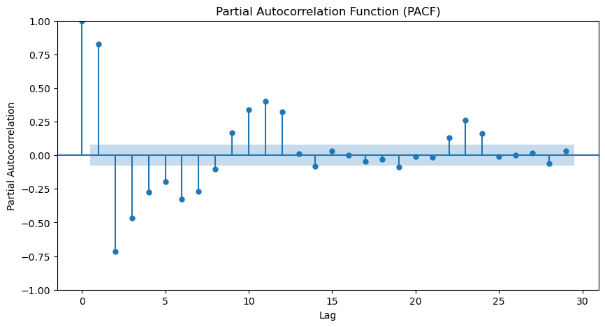
From the ACF and PACF, we can see a strong seasonality present in our data. From the ACF we can verify that the seasonal period is 12 as is expected due to our monthly data and a year having 12 months.
Before training our model we need to split our data into training and testing. For example, we could leave 2 years for forecasting and the remaining ones for training our model. This all depends on your specific objective.
# Split into training and testing
df_train = df_temp_max.loc[:'2020']
df_test = df_temp_max.loc['2021':]

# Plot the last 10 years of training data and the 2 of testing
ax = df_train[-12*10:].plot(figsize=(10, 5))
df_test.plot(ax=ax)
plt.legend(['Train', 'Test'])
plt.xlabel('Date')
plt.ylabel('Maximum temperature')
plt.show()
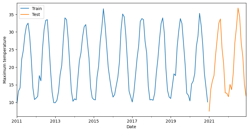
Once we have our training data ready we can proceed to train the model.
A SARIMA model is defined by 7 parameters as we mentioned before: (p, d, q)(P, D, Q, m) We know that our model does not need differencing to be stationary, therefore d will most likely be 0. Also, we know the seasonal period of our data is 12, so m will be 12.
Optimal model
We need to find the optimal model. What does this mean? The model must have enough prediction power while being as simple as possible to prevent overfitting the data.
For doing this we will iterate with all the reasonable combinations of parameters. This is called “grid search“. We need to fit each SARIMA model with the chosen parameter values to the training data and compare an evaluation metric.
Generally, the metric chosen is the AIC. AIC stands for Akaike Information Criterion. It is a statistical measure used to evaluate the quality of a model by balancing its goodness of fit with its complexity (number of parameters). The AIC is commonly used in model selection, including the selection of SARIMA models.
The AIC takes into account both the model’s ability to fit the data and the number of parameters used in the model. The formula for calculating AIC is as follows:
$$AIC = -2 \times \text{log-likelihood} + 2 \times k$$
where:
- log-likelihood represents the maximized log-likelihood of the model
- k is the number of parameters in the model
During the grid search, the AIC will be calculated for each model, the model with the lowest AIC value will indicate the best balance between accuracy and simplicity for your particular time series data.
Also, we need to bear in mind that we must keep only those models that converge. To ensure this we could just check the z-values, and ignore any models with any of them with an infinite value.
import itertools
import math

# Define the range of values for p, d, q, P, D, Q, and m
p_values = range(0, 3)  # Autoregressive order
d_values = [0]          # Differencing order
q_values = range(0, 3)  # Moving average order
P_values = range(0, 2)  # Seasonal autoregressive order
D_values = range(0, 1)  # Seasonal differencing order
Q_values = range(0, 2)  # Seasonal moving average order
m_values = [12]         # Seasonal period

# Create all possible combinations of SARIMA parameters
param_combinations = list(itertools.product(p_values,
                                            d_values,
                                            q_values,
                                            P_values,
                                            D_values,
                                            Q_values,
                                            m_values))

# Initialize AIC with a large value
best_aic = float("inf")
best_params = None

# Perform grid search
for params in param_combinations:
    order = params[:3]
    seasonal_order = params[3:]

    try:
        model = sm.tsa.SARIMAX(df_train,
                               order=order,
                               easonal_order=seasonal_order)
        result = model.fit(disp=False)
        aic = result.aic

        # Ensure the convergence of the model
        if not math.isinf(result.zvalues.mean()):
            print(order, seasonal_order, aic)

            if aic < best_aic:
                best_aic = aic
                best_params = params

        else:
            print(order, seasonal_order, 'not converged')

    except:
        continue

# Print the best parameters and AIC
print("Best Parameters:", best_params)
print("Best AIC:", best_aic)
Best Parameters: (2, 0, 1, 1, 0, 1, 12)
Best AIC: 2434.0270656007365
SARIMA model
Let’s then fit the model with the optimal parameters and check its summary.
model = sm.tsa.SARIMAX(df_train,
                       order=best_params[:3],
                       seasonal_order=best_params[3:])
result = model.fit(disp=False)

# Show the summary
result.summary()
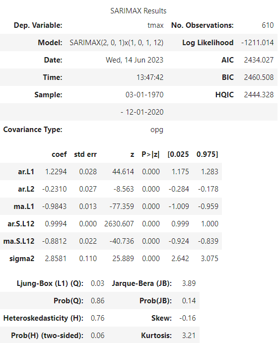
Let’s inspect the summary. We will focus on the coefficients part. Our SARIMA model has the following parameter estimates:
- The autoregressive terms (ar.L1 and ar.L2) have estimated coefficients of 1.2218 and -0.2248, respectively.
- The moving average term (ma.L1) has an estimated coefficient of -0.9846.
- The seasonal autoregressive term (ar.S.L12) has an estimated coefficient of 0.9988.
- The seasonal moving average term (ma.S.L12) has an estimated coefficient of -0.8444.
- The estimated variance of the error term (sigma2) is 2.9183.
The “P>|z|” column provides the p-value associated with each coefficient, for all cases they are lower than 0.05, our significance level, which means that all of them are statistically significant.
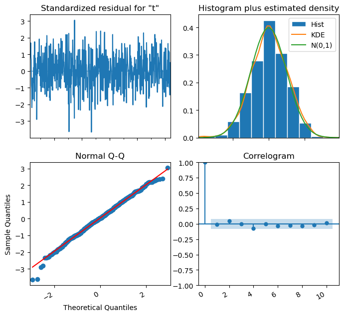
We can plot the model diagnostics to see if the model is a good fit.
For it to be considered as so, we need to meet the following requirements:
- The standardized residual shouldn’t have any obvious patterns. In this case we can just see random noise, data with a zero mean and a uniform variance, so this requirement is met.
- The histogram plus KDE estimate must look similar to a normal distribution. This is also met in our case.
- In the Normal Q-Q graph, we must observe the majority of the point lying on the straight line.
- In the ACF or correlogram, all lags must be within the confidence band. This is also met in our case.
We can then affirm that our model is a good fit for the data since the residuals are random noise following a normal distribution and there is no evidence of any patterns not captured by our model.
# Display the model diagnostics
fig = result.plot_diagnostics(figsize=(8, 8))
fig.autofmt_xdate()
plt.show()
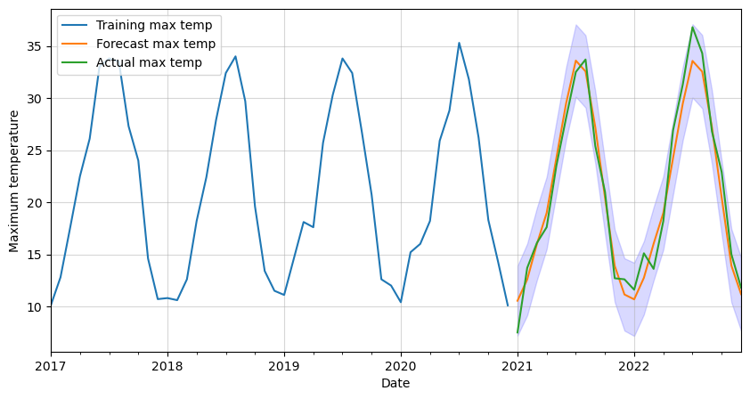
Finally, let’s forecast the maximum monthly temperature in Madrid for the next two years. We will also get the 95% confidence intervals and plot them all together. Two years in our data’s frequency is a total of 24 timesteps or steps.
# Get forecast and confidence intervals for two years
forecast = result.get_forecast(steps=24)
forecast_values = forecast.predicted_mean
confidence_intervals = forecast.conf_int()

# Plot forecast with training data
ax = df_train[-12*4:].plot(figsize=(10,5))
forecast_values.plot()
df_test.plot(ax=ax)
plt.fill_between(forecast_values.index,
                 confidence_intervals['lower tmax'],
                 confidence_intervals['upper tmax'],
                 color='blue',
                 alpha=0.15)
plt.legend(['Training max temp',
            'Forecast max temp',
            'Actual max temp'],
           loc='upper left')
plt.xlabel('Date')
plt.ylabel('Maximum temperature')
plt.grid(alpha=0.5)
plt.show()

If we want to check if our model is better or worse than another one, for example, Exponential Smoothing or Facebook Prophet, we could calculate some metrics and compare them. We will use the Mean Absolute Error (MAE), Root Mean Squared Error (RMSE), and Mean Absolute Percentage Error (MAPE).
# Predicted values and actual values
predicted_values = forecast_values.values
actual_values = df_test.values.flatten()

# Mean Absolute Error (MAE)
mae = np.mean(np.abs(predicted_values - actual_values))
print("MAE:", mae)

# Root Mean Squared Error (RMSE)
mse = np.mean((predicted_values - actual_values) ** 2)
rmse = np.sqrt(mse)
print("RMSE:", rmse)

# Mean Absolute Percentage Error (MAPE)
mape = np.mean(np.abs((predicted_values - actual_values) / actual_values)) * 100
print("MAPE:", mape)
MAE: 1.4675907357039788
RMSE: 1.6748468811463644
MAPE: 8.423398319153863
SARIMA model with AutoARIMA
There is an alternative to the previous optimization model called AutoARIMA. This allows us to find the optimal parameters and fit the resultant model in a faster and automatic way.
# Install the library if necessary
!pip install pmdarima

# Import the library
from pmdarima.arima import auto_arima

# Build and fit the AutoARIMA model
model = auto_arima(df_train,
                   seasonal=True,
                   m=12,
                   suppress_warnings=True)
model.fit(df_train)

# Check the model summary
model.summary()
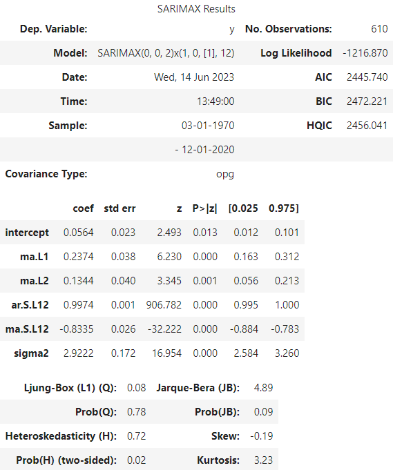
The first thing we observe is that AutoARIMA gave us a different optimal order. This is because it uses an approximation to speed up calculations. However, it may lead to a suboptimal model.
Let’s get the predictions and plot them. Remember to specify to return the confidence intervals by setting return_conf_int to True.
# Make predictions
forecast_auto, conf_int_auto = model.predict(n_periods=24,
                                             return_conf_int=True)

# Get forecast and confidence intervals for two years
forecast_values_auto = forecast_auto
confidence_intervals_auto = conf_int_auto

# Plot forecast with training data
ax = df_train[-12*4:].plot(figsize=(10,5))
forecast_auto.plot(ax=ax)
df_test.plot(ax=ax)
plt.fill_between(forecast_values_auto.index,
                 confidence_intervals_auto[:,[0]].flatten(),
                 confidence_intervals_auto[:,[1]].flatten(),
                 color='blue',
                 alpha=0.15)
plt.legend(['Training max temp',
            'Forecast max temp',
            'Actual max temp'],
           loc='upper left')
plt.xlabel('Date')
plt.ylabel('Maximum temperature')
plt.grid(alpha=0.5)
plt.show()
Let’s calculate the evaluation metrics for this model too.
# Predicted values and actual values
predicted_values_auto = forecast_auto.values
actual_values = df_test.values.flatten()

# Mean Absolute Error (MAE)
mae = np.mean(np.abs(predicted_values_auto - actual_values))
print("MAE:", mae)

# Root Mean Squared Error (RMSE)
mse = np.mean((predicted_values_auto - actual_values) ** 2)
rmse = np.sqrt(mse)
print("RMSE:", rmse)

# Mean Absolute Percentage Error (MAPE)
mape = np.mean(np.abs((predicted_values_auto - actual_values) / actual_values)) * 100
print("MAPE:", mape)
MAE: 1.4808593782629733
RMSE: 1.6965473977792707
MAPE: 8.446682735420076Model comparison
We can compare them with the ones obtained with the first SARIMA model.
| Metric | SARIMA | AutoARIMA |
|---|---|---|
| MAE | 1.4537 | 1.4811 |
| RMSE | 1.6545 | 1.6968 |
| MAPE | 8.3078 | 8.4488 |
Both are nearly identical, however, the first model is slightly better. This tells us that either approach should be perfectly valid for this case.
Finally, let’s plot them against each other and the testing data.
# Plot both forecasts against actual data
ax = forecast_values.plot(figsize=(10,5))
forecast_auto.plot(ax=ax)
df_test.plot(ax=ax)

plt.legend(['ARIMA max temp',
            'AutoARIMA max temp',
            'Actual max temp'],
           loc='lower right')
plt.xlabel('Date')
plt.ylabel('Maximum temperature')
plt.grid(alpha=0.5)
plt.show()
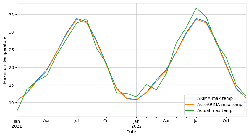
As we suspected, both models give a similar forecast.
For this particular example, we have forecasted a 24 months horizon. However, in some cases, only one step ahead would be necessary. In those cases using a rolling forecast approach would be more interesting. That would allow us to consider all the available information, and therefore improve our forecast.


0 Comments