Part I: Trend modeling

Classical time series forecasting techniques rely on statistical models that require a significant amount of effort to fine-tune and tailor to specific industry data. This often involves adjusting parameters to ensure accurate performance, which requires in-depth knowledge of the underlying models.

Prophet is an open-source library developed by Facebook designed to simplify the process of forecasting time series data, making it accessible to both analysts and non-experts.

Some of the main advantages of Prophet are:

• Due to its implementation in Stan, a statistical programming language written in C++, Facebook Prophet is extremely fast.
• Models are based on additive regression, which includes non-linear trends modeled with yearly, weekly, and daily seasonality. It is also possible to add a list of important holidays or events to the model.
• Prophet is designed to handle missing data, shifts in the trend, and outliers.
• It provides an easy procedure for tweaking and adjusting forecasts.

Assumptions

Like all time series forecasting models, Prophet makes several assumptions to model this data effectively:

• It assumes that the time series data has seasonality, which means that the patterns repeat periodically over time.
• It assumes that the time series data is stationary, which means that the statistical properties of the data do not change over time.
• It assumes that the time series data can be modeled using an additive model, which means that the trend, seasonality, and other components can be added together to get the overall forecast.
• It assumes that the trend component of the time series data follows a piecewise linear function, which means that the trend can change at different points in time.
• It assumes that overfitting should be avoided by setting appropriate priors on model parameters and using a validation set to evaluate the performance of the model.

Forecasting model

The Prophet forecasting model uses a decomposable time series model with three main components: trend, seasonality and holidays. This is similar to the approach followed by Exponential Smoothing models.

The following equation shows how they are combined:

$ y(t)= g(t) + s(t) + h(t) + \epsilon_t $

• $g(t)$: trend component
• $s(t)$: seasonal component
• $h(t)$: holidays or events component
• $\epsilon_t$: error term

Prophet approaches forecasting as a curve-fitting exercise, which contrasts with other time series models that explicitly consider the temporal dependence structure in the data. While this approach offers some benefits, such as flexibility and ease of use, it comes with some drawbacks, such as the lack of explicit incorporation of temporal dependencies in the model. As a result, Prophet may sacrifice some of the inferential advantages of a generative model, such as an ARIMA, which can capture the complex dependence patterns in the data and may provide more accurate and reliable forecasts.

Below you can find a basic example of how to train and use a Prophet model. Please note that Prophet expects the dataframe to have the following two columns:

• $ds$: the datestamp values
• $y$: the numeric measurement to forecast

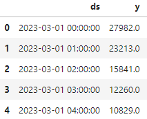
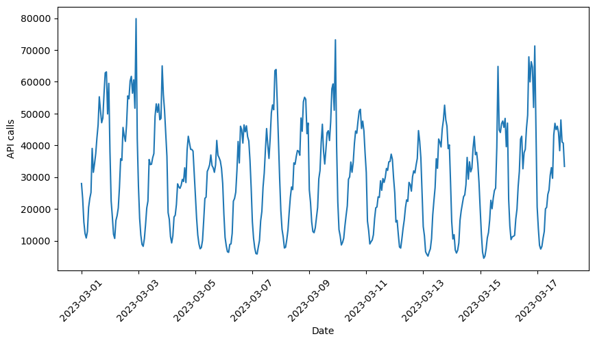
We can visualize the input data:

Following, a basic implementation of a Prophet model in Python:

# Import libraries
import pandas as pd
from prophet import Prophet

# Load data
df = pd.read_csv('dataset.csv')

# Instantiate model and fit data
model = Prophet()
model.fit(df)

# Define forecasting period
future = model.make_future_dataframe(periods=72,
                                     freq='H')
                                     
# Predict future values
forecast = model.predict(future)

# Plot forecast
fig = model.plot(forecast)

Note that the forecast horizon is specified here with the make_future_dataframe method. In this case set to 72 periods, which according to our frequency corresponds to 72 hours.

The different components can be shown with the following piece of code:

# Display the different components of the model
fig_2 = model.plot_components(forecast)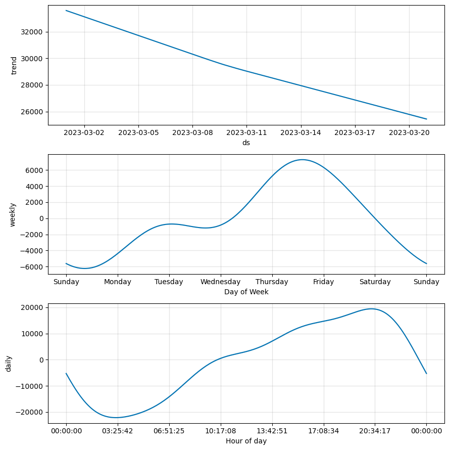

We will discuss the trend component in this article.

Trend

The trend component captures the non-periodic changes in a time series. This is built by fitting piecewise linear or logistic regression models to the data. These models are then combined to estimate the overall trend. To achieve this, Prophet segments the time series into smaller windows and applies a separate trend model to each window.

The rationale behind this approach is that time series data often exhibit abrupt changes in their patterns, and Prophet is designed to automatically detect these changepoints and adjust the trend accordingly. However, if greater precision is necessary, such as when Prophet misses a rate change or overfits the historical data, several input arguments are available to fine-tune the model.

How does Prophet deal with changes in trend?

Prophet can automatically detect changepoints in a time series data. It does so by first identifying a large number of possible changepoints. However, it tries to use as few of these changepoints as possible to avoid overfitting or underfitting.

The n_changepoints argument can be used to manually set the number of potential changepoints, but adjusting the regularization (changepoint_prior_scale) could be a better way to tune this.

# Set number of changepoints
model = Prophet(n_changepoints=30)

The significant changepoints can be visualized using add_changepoints_to_plot.

# Add changepoints to plot
from prophet.plot import add_changepoints_to_plot
fig = model.plot(forecast)
a = add_changepoints_to_plot(fig.gca(), model, forecast)

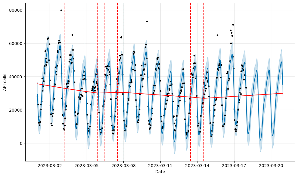
By default, changepoints are only inferred for the first 80% of the time series to avoid overfitting fluctuations at the end. However, this can be changed using the changepoint_range argument.

# Change changepoint range
model = Prophet(changepoint_range=0.9)

If the trend changes are being overfitted or underfitted, the changepoint_prior_scale argument (set by default to 0.05) can be used to improve it. It adds regularization to the changepoints effect. A higher value will make the trend more flexible, while a lower value will make it less flexible (damping the changepoints effect).

# Instantiate model and fit data
model = Prophet(changepoint_prior_scale=0.5)
model.fit(df)

It’s possible to manually specify the locations of potential changepoints using the changepoints argument, which will limit slope changes to those points only. A grid of points similar to the one generated by the automatic method could be combined with specific dates that are already known as possible changes. Alternatively, the changepoints could be limited to a small set of specific dates.

model = Prophet(changepoints=['2023-03-06', 
                              '2023-03-08', 
                              '2023-03-14'])

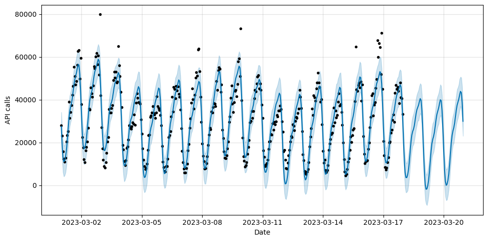
Linear model

The default trend model available in Prophet is a straightforward Piecewise Linear Model with a consistent growth rate, which is relatively easy to implement.

This model is most suitable for situations where a market cap or any other upper limit is not apparent, and can be set by specifying growth='linear' in the code. However, this is not necessary as it is the default model.

In cases where growth does not reach a saturation point, using a piece-wise constant growth rate can be a simple yet effective way to forecast future outcomes.

Logistic or saturating growth model

When predicting growth, there is typically a limit to how much it can reach, such as the total market size or population size. This limit is known as the carrying capacity, and any forecast should reach saturation at this point. It’s important to specify the carrying capacity, which is typically established using data or expert insights on the market size. To activate this model you should set growth='logistic' and specify the carrying capacity at the “cap” column of the dataset.

The logistic growth model is also capable of accommodating a minimum threshold that reaches a saturation point. This can be established using a “floor” column, similar to how the “cap” column sets the upper limit.

# Configure the model as a logistic growth model
model = Prophet(growth='logistic')
model.fit(df)

# Specify the carrying capacities in both df and future
df['cap'] = 100000
df['floor'] = 0
future['cap'] = 100000
future['floor'] = 5000

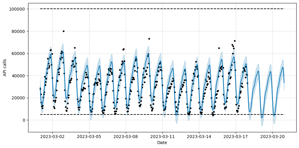
In this example, we have estimated that at least 5000 API calls will be received hourly in the next 72 hours. It is important to note that both the cap and floor must be specified when defining a minimum saturation point. Also, this must be set for both the historical data and the future dataframe.

In the next article, we will discuss the rest of the components used in Prophet models.

Time Series Forecasting with Facebook Prophet:

• Part I: Trend modeling
• Part II: Seasonality
• Part III: Exogenous variables