Part II: Seasonality

In the previous part of our Facebook Prophet series, we covered how to model the trend component and adjust the changepoints and regularization to improve forecasting accuracy. In this article, we’ll focus on the seasonal component and explore how to effectively model it using Facebook Prophet.

Seasonal component

The way Facebook Prophet uses to model seasonality is through partial Fourier sums. Partial Fourier sums are a truncated version of the Fourier series that uses a finite number of terms to represent a periodic function. The choice of how many terms to include in the partial Fourier sum depends on the desired level of accuracy in approximating the original function, in this case, the seasonal component of our time series data.

A higher order typically results in a more precise modeling of the periodic or seasonal component. However, as this component may not always be accurately estimated, reducing the order can lead to a smoother component and lessen the impact of significant seasonal changes.

_{Subscribe for free to our newsletter so you don’t miss any future articles!}

By default, Prophet fits yearly and weekly seasonality if the frequency of your data is daily or lower and if it is more than two cycles long. For the yearly component, the default Fourier order is 10, whereas for the weekly one it is 3. In addition, if your data has a time component then it will also fit a daily seasonality with the Fourier order set to 4.

We can fit a basic model as we did in the previous article.

# Import libraries
from prophet import Prophet

# Instantiate model and fit data
model = Prophet()
model.fit(df)

# Define forecasting period (daily by default)
future = model.make_future_dataframe(periods=72,
                                     freq='H')

# Predict future values
forecast = model.predict(future)

# Plot components
fig = model.plot_components(forecast)

We will get the following decomposition:

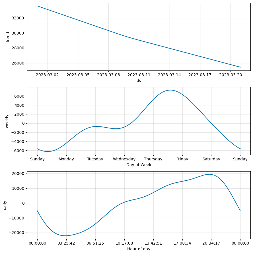
To confirm the default values, we can examine the “seasonalities” attribute of the model.

print(model.seasonalities)

OrderedDict([('weekly',
              {'period': 7,
               'fourier_order': 3,
               'prior_scale': 10.0,
               'mode': 'additive',
               'condition_name': None}),
             ('daily',
              {'period': 1,
               'fourier_order': 4,
               'prior_scale': 10.0,
               'mode': 'additive',
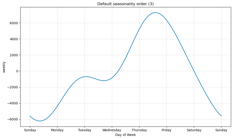
               'condition_name': None})])

You can check how the Fourier order affects the component modelling, for example, the weekly one:

from prophet.plot import plot_seasonality

# Plot default weekly seasonality order (3)
plot_seasonality(model, name='weekly')

# Plot increased weekly seasonality order
model = Prophet(weekly_seasonality=5).fit(df)
plot_seasonality(model, name='weekly')

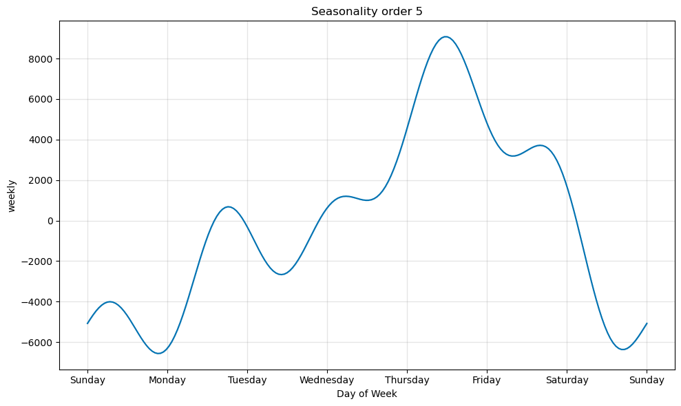
Ensure the Fourier order is not too high, otherwise, it may overfit your data or cause instabilities.

We could also switch off any non-desired seasonality, for example, the weekly one:

model = Prophet(weekly_seasonality=False)

If we are aware of another seasonality that Prophet is not considering by default, we could also add it. For example, we could add a monthly seasonality component. For this, we need to specify the component’s name, the period in days and the Fourier order.

# Add seasonality to instantiated model
model.add_seasonality(name='monthly',
                      period=30.5,
                      fourier_order=5)

Multiplicative seasonality

By default the seasonality considered by Prophet is additive. If you need the seasonality factor to grow with the trend you need to consider instead a multiplicative seasonality. You can specify it by doing the following:

model = Prophet(seasonality_mode='multiplicative')

This will make any seasonality, regressors and holidays be modelled as multiplicative. However, if you want some seasonality to be modeled as additive you can specify it when adding that seasonality component:

# Add seasonality to instantiated model
model.add_seasonality(name='monthly',
                      period=30.5,
                      fourier_order=5,
                      mode='additive')

Conditional seasonalities

Sometimes, the seasonality can be influenced by various factors, such as a daily pattern that varies between weekends and weekdays. It is possible that this could happen in our data, the daily seasonality could change since the amount of API calls may fluctuate based on the day of the week.

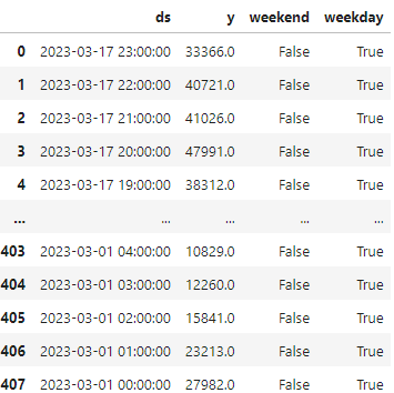
To begin, we can create a function that identifies whether a given date falls on a weekend (days 5 or 6) or a weekday (days 0 to 4). Next, we can leverage this function to generate two distinct features within our dataset: one indicating whether the date is weekend and the other indicating whether it is a weekday.

# Create a function that determines if it is weekend or not
def is_weekend(ds):
    date = pd.to_datetime(ds)
    return date.weekday() >= 5

# Create two features that indicate if it is weekend or not
df['weekend'] = df['ds'].apply(is_weekend)
df['weekday'] = ~df['ds'].apply(is_weekend)

We will obtain something like this:

Next, we need to reinstantiate the model while ensuring that we disable the daily seasonality to avoid having two equivalent seasonal patterns. We can incorporate seasonal variations for both weekdays and weekends.

We must add these features also in the “future” dataset following the same procedure. Once complete, we can fit the data and generate our predictions. We can finally plot the updated components.

# Instantiate the model without the daily seasonality
model = Prophet(daily_seasonality=False)

# Add the seasonality based on each condition
model.add_seasonality(name='daily_weekend',
                      period=1,
                      fourier_order=4,
                      condition_name='weekend')
                        
model.add_seasonality(name='daily_weekday',
                      period=1,
                      fourier_order=4,
                      condition_name='weekday')

# Add the condition to the future dataset too
future['weekend'] = future['ds'].apply(is_weekend)
future['weekday'] = ~future['ds'].apply(is_weekend)

# Fit the data and predict
forecast = model.fit(df).predict(future)

# Display the components
fig = model.plot_components(forecast)

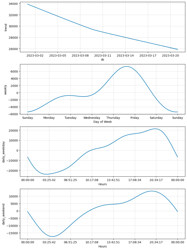
Now, we can compare both components to determine if there is similar behaviour on weekends and weekdays.

Add regularization

Sometimes the seasonal components may overfit the data. To reduce their influence we can adjust the prior scale. This will have a smoothing effect, damping the seasonality effect.

In certain cases, the seasonal components may result in overfitting. To address this, we can adjust the prior scale, which can serve to smooth out the seasonality effect and reduce its influence on the overall model. The default prior scale value is set to 10, to add regularization we can reduce this value.

We can affect all seasonal components by using the seasonality_prior_scale argument when instantiating the Prophet model.

model = Prophet(seasonality_prior_scale=0.01).fit(df)

We can also apply regularization to a specific seasonal component, in this case to the daily seasonality.

model.add_seasonality(name='daily',
                      period=1,
                      fourier_order=4,
                      prior_scale=0.01)

We can compare the daily seasonality effect with the default prior scale (10) and the one with a reduced one (0.01).

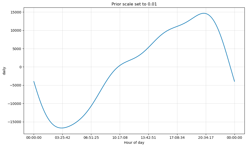
We can observe that the values for the second one are comparatively lower.

That is all about seasonality. In the next issue, we will cover events and exogenous variables or regressors.

Time Series Forecasting with Facebook Prophet:

• Part I: Trend modeling
• Part II: Seasonality
• Part III: Exogenous variables