Time series can be seasonal. What does this mean? It means that our data exhibits a season or cycle that regularly repeats, for example, weekly, monthly or annually.
There is something important to note. The presence of a cycle structure does not mean seasonality. For this cycle to be seasonal it needs to be consistently repeated at the same frequency. Otherwise, it is called a cycle, not a season.
Time series components
Time series data can be decomposed into different components:
- Trend or secular element: it is the long-term direction of the data
- Seasonal element: systematic, calendar-related variations. Consistently repeated at the same frequency.
- Cyclical element: periodical, but not seasonal variations.
- Residual or irregular element: unsystematic, short-term fluctuations. It is also called noise.
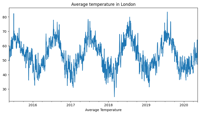
Example of seasonal time series data: Average temperature in London since 2016
Decomposition models
Time series data can include any of these components. However, not all of them include them in the same way. Let’s find out the most common models that take into account these elements. For simplicity, we will ignore the cyclical element.
Additive Model
These models assume the observed time series is the sum of its elements:
$$ y(t)=Trend+Seasonality+Residual $$
This model considers that the magnitudes of the seasonal and residual elements are independent of the trend.
Multiplicative Model
These models assume the observed time series is the product of its elements:
$$ y(t)=Trend×Seasonality×Residual $$
This model implies that the seasonality and residuals are dependent on the trend.
This model can be transformed into an additive model by applying logarithmic transformations:
$$ log(y(t))=log(Trend)+log(Seasonality)+log(Residual) $$
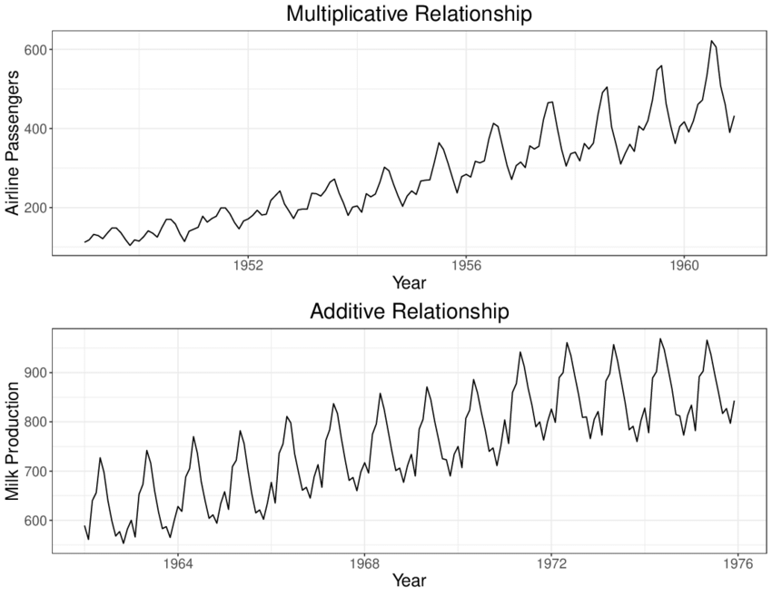
Additive and multiplicative decomposition models
Other models
In addition to the previous two models, there are other models that are also used to decompose time series data:
Pseudo-additive model
- Exponential smoothing
- Locally Estimated Scatterplot Smoothing (LOESS)
- Frequency-based methods
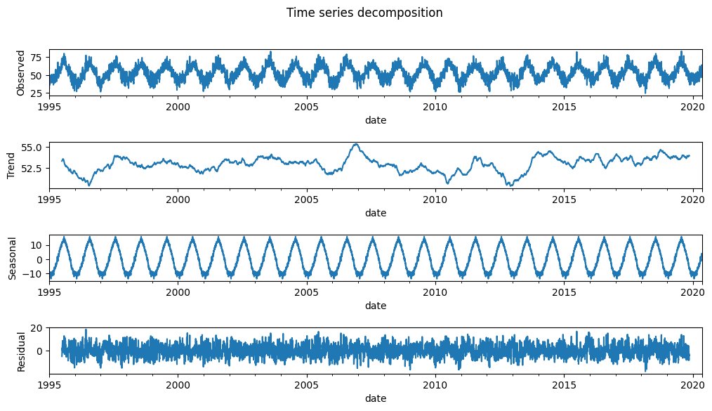
Time Series additive decomposition for the temperature in London since 1995
SARIMA model
In previous articles, we introduced the ARIMA model. This model is really useful when we don’t have seasonal variations. They can model the trend of the time series data.
However, if our data exhibits seasonality, we will require a Seasonal ARIMA model or so-called SARIMA. The SARIMA model is an extension of the ARIMA model to explicitly model the Seasonal component in univariate data.
A SARIMA(p,d,q)(P,D,Q)m model is defined by seven parameters. Three come from the ARIMA part and an additional four parameters characterize the modelling of the seasonal element:
Trend
- p : trend autoregressive order
- d : trend difference order
- q : trend moving average order
Seasonality
- P : seasonal autoregressive order
- D : seasonal difference order
- Q : seasonal moving average order
- m : number of timesteps for a seasonal period
Selection of parameters
The first parameter to choose is m. This must be chosen by inspecting the initial data and having some knowledge of what represents.
After knowing the number of timesteps of a single seasonal period, the data will be decomposed.
p and q will be selected as seen in the previous article by looking at the trend element using the ACF and PACF plots. d will be chosen so it makes the trend stationary.
In the same way, ACF and PACF plots are used to estimate the values of P and Q, by looking at the correlation of seasonal lags. D will be chosen to make a period of the seasonal element stationary.
However, you can just use auto-ARIMA once you have the frequency m to select the last six parameters.
Limitations
The limitation of the SARIMA models is that they can be used only with single seasonality. For example, there could be cases in which we could have seasonality during the day, during the week and also during the year. There are other models able to deal with that, for instance: TBABS.
Try it yourself!
Decompose your data
If you want to decompose some time series data, you can follow the step-by-step guide in the following Kaggle notebook:

Build your Auto-ARIMA model
Here you have a guide on how to automatically build your own optimal ARIMA model:
Time Series articles
- Introduction to ARIMA models
- Parameters selection in ARIMA models
- Seasonal ARIMA
- ARCH / GARCH models for Time Series
- ARIMA-GARCH models


0 Comments