Exponential Smoothing for Time Series Forecasting

Exponential Smoothing is a popular time series forecasting method used for univariate data. While other methods, such as ARIMA models, develop a model based on a weighted linear sum of recent past observations or lags, Exponential Smoothing models employ an exponentially decreasing weight for past observations.

This weight is calculated using a geometrically decreasing ratio, which means that the more recent observations are given greater weight in the prediction than older observations. This approach helps to reduce the impact of outliers and noise in the data and provides a more accurate prediction.

Types

There are three types of Exponential Smoothing models. These models differ based on the assumptions they make about the data. The three types are:

1. Simple exponential smoothing
2. Double exponential smoothing
3. Triple exponential smoothing

Collectively, these models are referred to as ETS models, which stands for “Error, Trend, and Seasonality”. ETS models explicitly model the three key components that can affect time series data. Each type of smoothing model builds upon the previous one by adding an additional element to the forecasting process. Therefore, simple exponential smoothing only considers the error term, double exponential smoothing takes both error and trend into account, and triple exponential smoothing adds seasonality to the mix.

The added elements increase the complexity of the model, but also enhance its ability to capture the underlying patterns in the data and provide more accurate forecasts.

Simple Exponential Smoothing

This model is used to model the level of the data. Suitable for forecasting data that lacks any systematic structure, such as a clear trend or seasonality. Therefore it is assumed that data is stationary.

Its equation of the Simple Exponential Smoothing model is:

$$ y_{t+1} = α x_{t}+(1-α) y_{t} $$

• $y_{t+1}$: forecasted value
• $y_{t}$: previous period forecast
• $x_{t}$: observed value
• $\alpha$: smoothing constant for the level

You can see that there is only one parameter, $\alpha$, which corresponds to the smoothing or weighting constant for the level and it ranges from 0 to 1. Large values (close to 1) mean that the model will pay more attention to the most recent observations. Small values (close to 0) mean that the forecast will have a larger influence by past observations.

There is no need for a manual implementation since the statsmodels library in Python includes this model: statsmodels.tsa.holtwinters.SimpleExpSmoothing

Let’s see an example, in which we will forecast the next 5 periods of our data, corresponding to the millions of international visitor nights in Australia in the next five quarters of the year:

data = [
    41.7275,
    24.0418,
    32.3281,
    37.3287,
    46.2132,
    29.3463,
    36.4829,
    42.9777,
    48.9015,
    31.1802,
    37.7179,
    40.4202,
    51.2069,
    31.8872,
    40.9783,
    43.7725,
    55.5586,
    33.8509,
    42.0764,
    45.6423,
    59.7668,
    35.1919,
    44.3197,
    47.9137,
]
index = pd.date_range(start="2005", end="2010-Q4", freq="QS-OCT")
aust = pd.Series(data, index)

from statsmodels.tsa.api import SimpleExpSmoothing

forecast_period = 5
train_data = aust.iloc[:-forecast_period]

# Fit data 
model = SimpleExpSmoothing(train_data, 
    initialization_method="heuristic").fit(
    smoothing_level=0.2, 
    optimized=False
)

# Forecast following 5 periods
forecast = model.forecast(forecast_period)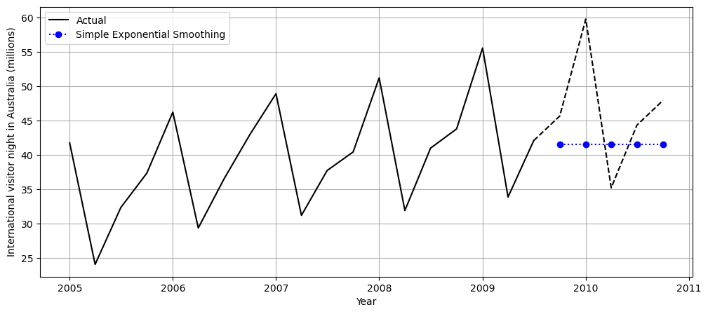

You can see that the forecasting is a horizontal line. This model is only capable of predicting the level component.

Double Exponential Smoothing

It is an extension of the previous type that adds support for modelling the trend. Therefore, it is suitable for data with a trend but no seasonality. There can be two kinds of models, depending on the type of trend:

• Additive trend (Holt’s linear trend model): Double Exponential Smoothing with a linear trend.
• Multiplicative Trend: Double Exponential Smoothing with an exponential trend.

The set of equations for the additive trend model is:

$\text{Model:}$

$y_{t+n} = l_t+n b_t $

$\text{Level:}$

$l_t = α x_{t}+(1-α) (l_{t-1}+b_{t-1}) $

$\text{Trend: }$

$ b_t = \beta (l_t-l_{t-1}) +(1-\beta) b_{t-1}$

The set of equations for the multiplicative trend model is:

$\text{Model:}$

$y_{t+n} = l_t r_t^n $

$\text{Level:}$

$l_t = α x_{t}+(1-α) (l_{t-1} r_{t-1}) $

$\text{Growth rate: }$

$ r_t = \beta \dfrac{l_t}{l_{t-1}}+(1-\beta) r_{t-1}$

This model adds the following variables:

• $l_{t}$: level value at period $t$
• $b_{t}$: trend value at period $t$. Only for additive trend models.
• $r_{t}$: growth rate value at period $t$. Only for multiplicative trend models.
• $\beta$: smoothing constant for the trend
• $n$: number of periods to forecast

In this case, we have two smoothing constants: $\alpha$ and $\beta$, one for the level and one for the trend. Similarly to $\alpha$, $\beta$ ranges from 0 to 1, with small values meaning a higher influence of past observations and large values a higher influence of recent observations.

This model is also available thanks to the statsmodels library in Python: statsmodels.tsa.holtwinters.Holt

We can use this model to try to get a better forecast than the one done with the Simple Exponential Smoothing model:

from statsmodels.tsa.api import Holt

forecast_period = 5
train_data = aust.iloc[:-forecast_period]

# Fit data 
model = Holt(train_data, 
    exponential=True, 
    initialization_method="estimated").fit(
    smoothing_level=0.2, 
    smoothing_trend=0.1, 
)

# Forecast next 5 periods
forecast = model.forecast(forecast_period)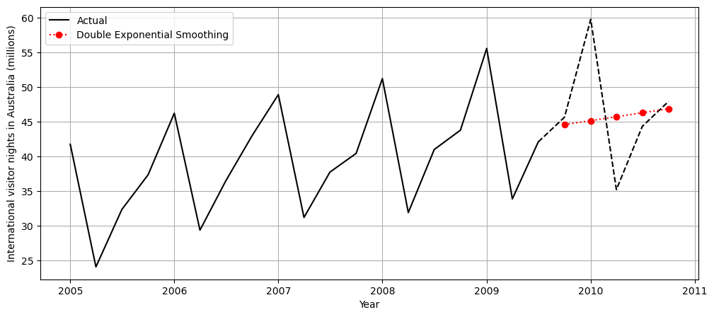

This model is capable of forecasting both the level and the trend. We can see how the forecasting has a slope.

Triple Exponential Smoothing

This type extends the previous model by adding support for modelling the seasonal component. Therefore, it is suitable for data with a trend and seasonality. It is also called Holt-Winters Exponential Smoothing. As with the Double Exponential Smoothing model, we need to distinguish two kinds of models, depending on the type of seasonal component, in addition to the two variations depending on the type of trend:

• Additive Seasonality: Triple Exponential Smoothing with a linear seasonality.
• Multiplicative Seasonality: Triple Exponential Smoothing with an exponential seasonality.

For simplicity, we will show the equations for the model with an additive trend.

The set of equations for the additive seasonality model is:

$\text{Model:}$

$y_{t+n} = l_t + n b_t + c_{t+n-s}$

$\text{Level:}$

$l_t = α (x_{t}-c_{t-s}) + (1-α) (l_{t-1} + b_{t-1}) $

$\text{Trend: }$

$ b_t = \beta (l_t-l_{t-1}) + (1-\beta) b_{t-1}$

$\text{Seasonality:}$

$ c_t = \gamma(x_t-l_{t}) + (1-\gamma) c_{t-s}$

The set of equations for the multiplicative seasonality model is:

$\text{Model:}$

$y_{t+n} = (l_t + n b_t) c_{t+n-s}$

$\text{Level:}$

$l_t = α (x_{t}-c_{t-s}) + (1-α) (l_{t-1} + b_{t-1}) $

$\text{Trend: }$

$ b_t = \beta (l_t-l_{t-1}) + (1-\beta) b_{t-1}$

$\text{Seasonality:}$

$ c_t = \gamma \dfrac{x_t}{l_{t}} + (1-\gamma) c_{t-s}$

The additional variables that the Holt-Winters model incorporates are:

• $c_{t}$: seasonality value at period $t$
• $s$: seasonal periods
• $\gamma$: smoothing constant for the seasonality

Here we have three smoothing constants: $\alpha$, $\beta$ and $\gamma$, one for the level, one for the trend and one for the seasonality. $\gamma$ also ranges from 0 to 1 and works in a similar way.

Note that by simplifying $b_t$ and $c_t$ you can go from a Triple Exponential Smoothing model to a Simple Exponential Smoothing one. Each model type just adds an extra element to the previous type.

You can use this model with the library statsmodels in Python: statsmodels.tsa.holtwinters.ExponentialSmoothing

Let’s see an example with this model type:

from statsmodels.tsa.api import ExponentialSmoothing

forecast_period = 5
train_data = aust.iloc[:-forecast_period]

# Fit data 
model = ExponentialSmoothing(
    train_data,
    seasonal_periods=4,
    trend="add",
    seasonal="add",
    use_boxcox=True,
    initialization_method="estimated",
).fit()

# Forecast next 5 periods
forecast = model.forecast(forecast_period)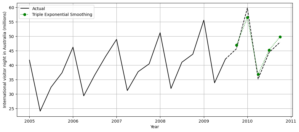

Finally, we observe how this model is capable of forecasting the level, the trend and the seasonality.

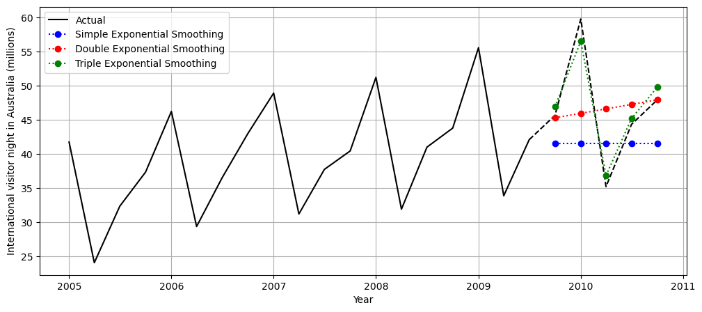
We can also overlap the three forecastings to see how they compare:

Optimizing the model

The effectiveness of these models depends on selecting the appropriate smoothing factors and time period:

• If the smoothing factors are too high, the model may overreact to recent changes in the data and produce an unstable forecast. On the other hand, if the smoothing factors are too low, the model may not respond quickly enough to changes in the data, resulting in a lagged forecast.
• Similarly, choosing the appropriate time period is crucial for capturing any seasonal patterns in the data.

By selecting appropriate values for the smoothing factor and time period, one can achieve the best results from the exponential smoothing method.

Damping

In addition to the smoothing factors, both Double and Triple Exponential Smoothing models can also include the $\phi$ damping coefficient to control the rate of growth of the trend over future time steps.

The damping coefficient is a value generally between 0 and 1, where a value closer to 1 indicates a slower growth rate, and a value closer to 0 indicates a faster growth rate. A value of 1 indicates no damping, and the trend component grows linearly without any damping effect. In contrast, a value of 0 implies a completely damped trend, and the forecast remains constant over time. A damping coefficient value greater than 1 or less than 0 can cause the forecast to become unstable.

Therefore, selecting an appropriate damping coefficient is important to ensure stable and accurate forecasts.

Conclusion

Exponential Smoothing models have a range of advantages that make them a popular choice for time series analysis. They are easy to understand, explainable, and can handle non-stationary data and small datasets. With a relatively small set of hyperparameters and lower time complexity, Exponential Smoothing models are fast and efficient, making them a suitable choice for time series analysis when computational resources are limited.

However, it is important to note that the choice of model depends on the specific characteristics of the time series being analyzed, and in some cases, other models like ARIMA may be more suitable for handling long-term trends and nonlinear dependencies.