Clean your Time Series data II: Remove seasonality and normalize data

In the first part of this series, we saw that cleaning the data is an essential step in the time series analysis process. This consists of the following substeps:

1. Handle missing values
2. Remove trend
3. Remove seasonality
4. Check for stationarity and make it stationary if necessary
5. Normalize the data
6. Remove outliers
7. Smooth the data

The article will provide a general guideline for removing the seasonality and normalizing the time series data. Please remember that depending on your data, you will need to skip some steps or modify or add other ones.

Remove seasonality

Before starting, we could use Python’s statsmodels library to see the seasonal decomposition of the data before we removed the trend. This is not a required step, but it could be useful to visualize the components of the time series data. Before using it, we need to select the seasonality period. Since we are working with monthly beer production, we can assume that the data will have some kind of seasonality during the year and that this should be repeated over the years. Therefore, our period will be set to 12 (referring to 12 months since we have a monthly frequency in our data and we assumed an annual seasonality).

# Import library
import statsmodels.api as sm

# Decompose data by selecting the appropiate frequency
decomp = sm.tsa.seasonal_decompose(
  df['Monthly beer production'], period=12)
decomp_plot = decomp.plot()

# Plot outcome
plt.xlabel('Date')
decomp_plot .set_figheight(10)
decomp_plot .set_figwidth(10)
plt.show()

As expected, we can see one production peak every year and a smooth trend without ups and downs, only the actual trend over the years. We can also see the residuals, which refer to all noise or anomalies during this period of time after extracting the seasonal component and the trend.

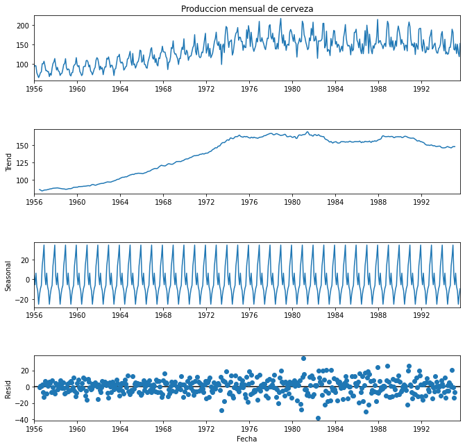
We must pay attention to the magnitude of the different components. On the one hand, the trend must be large compared to the seasonal component, but the seasonal component must be relevant and large enough to be able to say that there is seasonality. On the other hand, the majority of values of the residuals must be small and randomly distributed, however, some large values may still appear in those cases where there is a clear outlier. We can say that this is the behaviour we observe in our data.

One way of getting rid of the seasonality and also smoothing the data could be taking into consideration only the trend component. We will just need to remember to add this component later after we do the forecast!

Another possibility could be not doing anything with the seasonality, and leaving it within the data. In this case, we would need to use a model capable to handle seasonality such as SARIMA.

However, if we are going to use a Machine Learning approach, possibly removing it now will be the most logical step. We will use a more intuitive approach for this.

# Calculate each year's average
monthly_average = df_beer.groupby(df_beer.index.month).mean()
mapped_monthly_average = df_beer.index.map(
    lambda x: monthly_average.loc[x.month])

# Standardize each year's average
df_beer = df_beer / mapped_monthly_average

# Plot outcome
df_beer.plot(figsize=(15,5))
plt.xlabel('Date')
plt.ylabel('Standardized beer production rate')
plt.grid()
plt.show()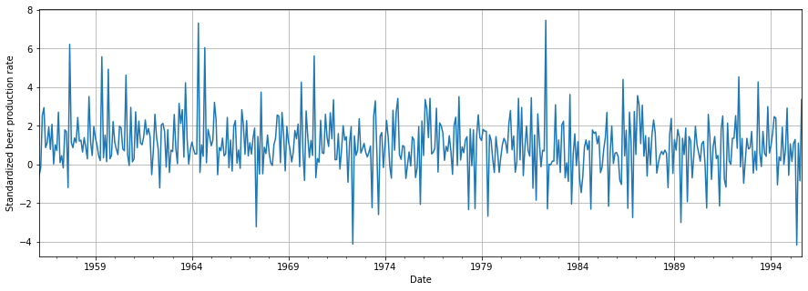

We can see now that the outcome looks pretty random and therefore stationary. We could check if this is actually the case.

Check for stationarity

Stationarity refers to a property of the data where statistical properties such as the mean, variance, and autocorrelation structure remain constant over time. In other words, a stationary time series has a constant mean, constant variance, and its autocovariance does not depend on time.

This property is important because it allows us to model the underlying process generating the data and make predictions based on that model. Non-stationarity, on the other hand, can make it difficult to model and forecast the data, as the statistical properties of the time series can change over time.

There are a few statistical tests that can be used to check for stationarity in a time series. But first, we need to introduce what a unit root is. A unit root refers to a value of the parameter in the autoregressive (AR) model that is equal to one. The two main tests to check for stationarity are:

• Augmented Dickey-Fuller (ADF) test: It is used to check for the presence of a unit root in the time series data, which is a common cause of non-stationarity. The null hypothesis ($H_0$) is that the data is non-stationary, and a rejection of this hypothesis indicates that the data is stationary.
• Kwiatkowski-Phillips-Schmidt-Shin (KPSS) test: This test is used to check for the presence of a trend in the data, which can also cause non-stationarity. The null hypothesis ($H_0$) is that the data is stationary, and a rejection of this hypothesis indicates the presence of a trend.

Note that the null hypotheses for these two tests are contrary, therefore we will need to be careful when interpreting the p-values.

Let’s perform both tests using the functions in statsmodels library:

# Import required libraries
from statsmodels.tsa.stattools import adfuller, kpss

# Perform ADF test
result = adfuller(df_beer)
print('ADF test:\tp-value: {:.3f}'.format(result[1]))

# Perform KPSS test
result = kpss(df_beer)
print('KPSS test:\tp-value: {:.3f}'.format(result[1]))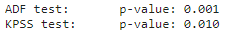

For the KPSS test, we need to check if the p-value is greater than the significance level. In this case, it is lower than 0.05, therefore it is not stationary according to this test.

We still need to work on making our data stationary. We can simply apply another differencing and perform both tests again.

# Apply one more differencing to the data
df_beer = df_beer.diff()[1:]

# Perform ADF test
result = adfuller(df_beer)
print('ADF test:\tp-value: {:.3f}'.format(result[1]))

# Perform KPSS test
result = kpss(df_beer)
print('KPSS test:\tp-value: {:.3f}'.format(result[1]))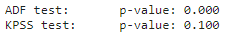

Normalize the data

The next step is to bring the data to a common scale, this is called normalization. There are different techniques:

1. Min-Max Scaler: This scaler scales each feature to a given range, typically between 0 and 1. It’s useful when you want to preserve the shape of the original distribution but adjust the scale of the data.
2. Standard Scaler: This scaler scales the data to have zero mean and unit variance. It is equivalent to calculating the z-score of the data. It’s useful when the distribution of the data is not normal and you want to normalize it to a standard Gaussian distribution.
3. Robust Scaler: This scaler is robust to outliers in the data and scales the data to the IQR (interquartile range). It’s useful when you have data with extreme values that could skew the scaling process.
4. Max-Abs Scaler: This scaler scales each feature to the maximum absolute value of that feature. It’s useful when the data is centered around zero, and you want to preserve the direction and sign of each feature.

We will use the Standard Scaler, since it will be useful later for removing the outliers. There are two alternatives here: the intuitive approach and the one using the scikit-learn library.

The intuitive approach is very easy and straightforward to implement:

# Calculate mean and standard deviation
mean = df_beer.mean()
std = df_beer.std()

# Normalize data
df_beer = (df_beer - mean) / std

We can also achieve the same outcome with the scikit-learn function:

# Import library
from sklearn.preprocessing import StandardScaler

# Create a StandardScaler object
scaler = StandardScaler()

# Convert data to numpy array and reshape
array_beer = df_beer.values.reshape(-1, 1)

# Fit the scaler to the data and transform it
data_scaled = scaler.fit_transform(array_beer)

# Convert back to pandas Series
df_beer = pd.Series(data_scaled.flatten(), 
                    index=df_beer.index, name='Month')

Both results will be the same. Two considerations:

• If you opt for the scikit-learn approach, you will be able to easily test other techniques simply by replacing StandardScaler by MinMaxScaler, MaxAbsScaler or RobustScaler.
• Make sure you keep the mean and standard deviation values in the first approach and the scaler object in the second for being able to go back to the beer production values after getting the forecast from the model.

We can display how the normalized data looks like:

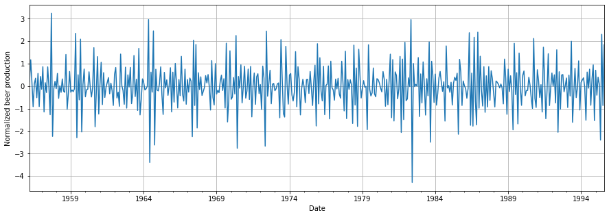
We can finally see how our data is stationary and normalized. We are now a step closer to being able to start building our model!

See all the parts of the data cleaning series:

1. Missing values and detrending
2. Remove seasonality and normalize data
3. Outliers removal
4. Data Smoothing

You can access the notebook in our repository:

GitHub – MLPills/remove-seasonality-and-normalize-data: A Jupyter Notebook that covers the basics of removing seasonality, making the data stationary and normalizing data

A Jupyter Notebook that covers the basics of removing seasonality, making the data stationary and normalizing data – GitHub – MLPills/remove-seasonality-and-normalize-data: A Jupyter Notebook that covers the basics of removing seasonality, making the data stationary and normalizing data

github.com

To run it right now click on the icon below:

We will see in the next article how we can check and remove outliers!