Granger Causality in Time Series Forecasting

We talked about Vector Autorregression or VAR in a previous article. But, does it really make sense to use two different variables to get a forecast? The answer is no, not always at least. It will only be beneficial if there is some kind of relationship between them. Using unrelated variables could introduce noise and confusion into the model, hindering accurate predictions rather than enhancing them.

A straightforward way of checking whether there is any relationship between the variables could be by computing the correlation. But this is not the only type of relationship that two variables can have.

We could also check if there is some kind of causation relationship between the variables. However, there is something essential to understand first, that our tests show causation doesn’t necessarily mean that one is the cause of the other, simply that there is some kind of correlation.

Let’s deep dive into this with an example about COVID.

Data: COVID cases and deaths in Germany

Let’s first import the data and do some basic processing. We will use COVID data from Germany. The data is split by state, county, age, and gender; but for the sake of simplicity, we will group it together.

# Read csv file
df_input = pd.read_csv('/kaggle/input/covid19-tracking-germany/covid_de.csv')

# Convert the date column to datetime
df_input['date'] = pd.to_datetime(df_input.date, format='%Y-%m-%d')

# Group the data by day and keep only number of cases and deaths
df = df_input.groupby(['date']).sum()[['cases', 'deaths']]

# Display data
df.plot(figsize=(10,5))
plt.grid(alpha=.3)
plt.ylabel('Number of cases/deaths')
plt.show()

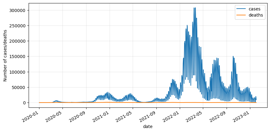
Data processing

The number of deaths are way smaller than the cases, so let’s bring both variables to a similar scale by applying a standard scaler.

from sklearn.preprocessing import StandardScaler

# Instantiate model
scaler = StandardScaler()

# Fit and transform, and format it as dataframe
df_scaled = pd.DataFrame(scaler.fit_transform(df), 
                         columns=df.columns, 
                         index=df.index)

# Visualize outcome
df_scaled.plot(figsize=(10,5))
plt.grid(alpha=.3)
plt.ylabel('Scaled number of cases/deaths')
plt.show()

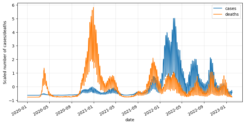
Now we can notice that the data is really noisy. What we can do is smooth it by applying a rolling average with a period of 7 (a week).

# Apply a rolling average of 7 days
df_roll = df_scaled.rolling(7).mean().dropna()

# Plot results
df_roll.plot(figsize=(10,5))
plt.grid(alpha=.3)
plt.ylabel('Scaled number of cases/deaths')
plt.show()

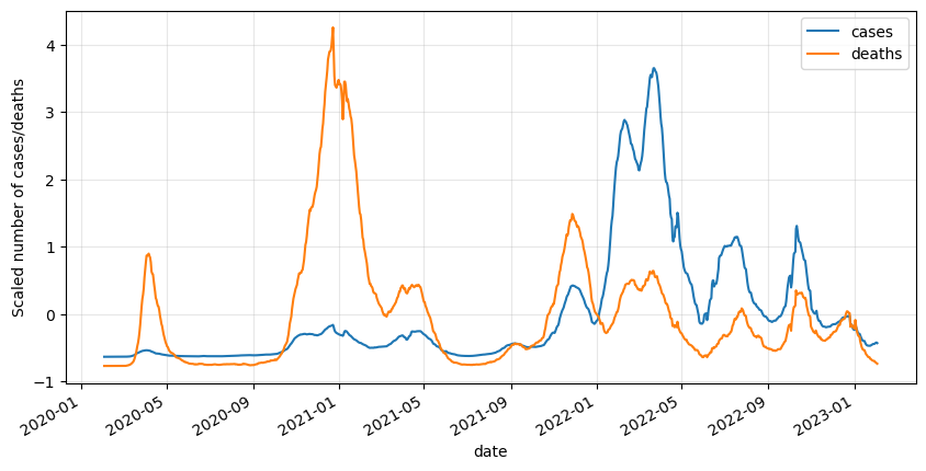
This graph looks much better now, time to start finding a relationship between cases and deaths!

Correlation

When examining correlation between variables, it is generally recommended to work with stationary variables rather than the original non-stationary series or after differencing. This is because correlation is a measure of linear association between variables, and non-stationary variables can exhibit trends or seasonality that can lead to spurious correlations.

Make data stationary

So let’s first apply a differencing to the variables to make them stationary.

# Apply differencing
df_diff = df_roll.diff().dropna()

# Plot results
df_diff.plot(figsize=(10,5))
plt.grid(alpha=.3)
plt.ylabel('Scaled increment of cases/deaths')
plt.show()

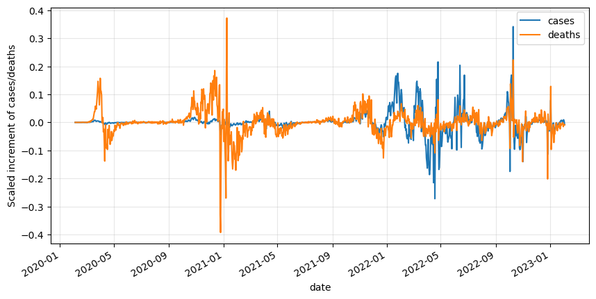
Let’s apply an Augmented Dickey-Fuller (ADF) test to verify the stationarity assumption after differencing.

from statsmodels.tsa.stattools import adfuller

for variable in df_diff.columns:

    # Perform the ADF test
    result = adfuller(df_diff[variable])

    # Extract and print the p-value from the test result
    p_value = result[1]
    print("p-value:", p_value)

    # Interpret the result
    if p_value <= 0.05:
        print(f"The variable {variable} is stationary.\n")
    else:
        print(f"The variable {variable} is not stationary.\n")

p-value: 9.530072056006194e-12
The variable cases is stationary.

p-value: 4.2719685376631305e-05
The variable deaths is stationary.

Both p-values are lower than 0.05, therefore we can assume they are stationary. We have verified that now they are both stationary.

Test for correlation

We are ready to check if there is any correlation between variables.

# Check correlation
df_diff.corr()

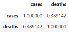
We get that there is some positive correlation (0.389) between variables. That means that using one to forecast the other may be useful.

However, there are other ways of seeing if there is any relationship between the variables since there is not always a correlation. We can also test for the so-called Granger causality.

Granger causality

Granger causality is a statistical concept that helps determine whether one variable can be used to predict another variable. It provides a way to measure the causal relationship between two time series variables.

Granger causality, like other statistical tests for causation, does not establish a true cause-and-effect relationship between variables. Instead, it provides evidence of potential causality based on the statistical association between the variables. It does not necessarily imply a true cause-and-effect relationship.

Granger causality is based on the idea that if variable X “Granger-causes” variable Y, then past values of X should contain information that helps predict future values of Y beyond what can be predicted by the past values of Y alone.

When conducting the Granger’s causality test, you estimate two regression models: one that includes the lagged values of both X and Y as predictors and another that only includes the lagged values of Y. By comparing the fit of these two models, you can assess whether including the lagged values of X improves the prediction of Y.

If the inclusion of lagged values of X significantly improves the prediction of Y compared to the model without X, then it suggests that X has some “Granger-causal” influence on Y. This means that X contains useful information for forecasting Y beyond what Y’s own past values provide.

Test for Granger causality

Let’s check if the deaths and the cases are Granger-causing each other. Causality tests must be applied to stationary variables, as otherwise, it can lead to spurious relationships, as they may reflect common trends rather than true causal links.

We will check Granger causality for the first 3 lags. First, we will see if deaths cause cases. We do this by setting deaths as the second column in the input dataframe, and cases as the first one.

from statsmodels.tsa.stattools import grangercausalitytests
​
# Check deaths as a Granger-cause 
deaths_as_cause = grangercausalitytests(df_diff[['cases', 'deaths']], 3)

Granger Causality
number of lags (no zero) 1
ssr based F test:         F=0.0000  , p=0.9985  , df_denom=1083, df_num=1
ssr based chi2 test:   chi2=0.0000  , p=0.9985  , df=1
likelihood ratio test: chi2=0.0000  , p=0.9985  , df=1
parameter F test:         F=0.0000  , p=0.9985  , df_denom=1083, df_num=1

Granger Causality
number of lags (no zero) 2
ssr based F test:         F=1.2480  , p=0.2875  , df_denom=1080, df_num=2
ssr based chi2 test:   chi2=2.5075  , p=0.2854  , df=2
likelihood ratio test: chi2=2.5046  , p=0.2858  , df=2
parameter F test:         F=1.2480  , p=0.2875  , df_denom=1080, df_num=2

Granger Causality
number of lags (no zero) 3
ssr based F test:         F=0.1804  , p=0.9097  , df_denom=1077, df_num=3
ssr based chi2 test:   chi2=0.5448  , p=0.9089  , df=3
likelihood ratio test: chi2=0.5447  , p=0.9090  , df=3
parameter F test:         F=0.1804  , p=0.9097  , df_denom=1077, df_num=3

Now we will check whether cases cause deaths. We do this by changing the order of the columns of the input dataframe.

# Check cases as a Granger-cause 
cases_as_cause = grangercausalitytests(df_diff[['deaths', 'cases']], 3)

Granger Causality
number of lags (no zero) 1
ssr based F test:         F=4.7868  , p=0.0289  , df_denom=1083, df_num=1
ssr based chi2 test:   chi2=4.8000  , p=0.0285  , df=1
likelihood ratio test: chi2=4.7894  , p=0.0286  , df=1
parameter F test:         F=4.7868  , p=0.0289  , df_denom=1083, df_num=1

Granger Causality
number of lags (no zero) 2
ssr based F test:         F=16.8184 , p=0.0000  , df_denom=1080, df_num=2
ssr based chi2 test:   chi2=33.7926 , p=0.0000  , df=2
likelihood ratio test: chi2=33.2770 , p=0.0000  , df=2
parameter F test:         F=16.8184 , p=0.0000  , df_denom=1080, df_num=2

Granger Causality
number of lags (no zero) 3
ssr based F test:         F=10.5894 , p=0.0000  , df_denom=1077, df_num=3
ssr based chi2 test:   chi2=31.9746 , p=0.0000  , df=3
likelihood ratio test: chi2=31.5121 , p=0.0000  , df=3
parameter F test:         F=10.5894 , p=0.0000  , df_denom=1077, df_num=3

How do we interpret these results?

The p-value we should primarily focus on is the one associated with the “ssr based F test” or the “likelihood ratio test.” These tests examine the null hypothesis that the lagged values of one variable do not have a significant effect on predicting the other variable.

Let’s introduce the hypotheses of this test:

• H0 (Null Hypothesis): The lagged values of one variable do not have a significant effect on predicting the other variable. In other words, there is no Granger causality between the two variables.
• H1 (Alternative Hypothesis): The lagged values of one variable have a significant effect on predicting the other variable. In other words, there is evidence of Granger causality between the two variables.

If the p-value is less than 0.05, we should reject the null hypothesis, which would suggest that there is evidence of Granger causality at a 5% significance level. This means that the lagged values of one variable have a significant effect on predicting the other variable.

According to these tests, deaths do not Granger-cause cases, but cases do Granger-cause deaths. This is exactly what we expected. Therefore, a VAR model can be helpful in this case.

What if there is only one-way Granger causality?

A VAR model can still be used even if only one variable shows Granger causality over the other variables. In a VAR model, each variable is treated as an endogenous variable, and the model captures the dynamic relationships between them.

If only one variable shows significant Granger causality over the others, it suggests that this variable has predictive power in explaining the variations in the other variables. This information can still be valuable in understanding the system’s dynamics and forecasting future values.

However, it is important to interpret the results carefully. The presence of significant Granger causality from one variable to others indicates a potential causal relationship, but it does not necessarily imply complete and deterministic causation.

What if there is no Granger causality?

A VAR model can still be useful even if no Granger causality is found between the variables. The absence of significant Granger causality suggests that the past values of one variable do not provide substantial additional information in predicting the future values of another variable beyond what is already captured by the lagged values of that variable itself. In such cases, a VAR model can still capture the contemporaneous relationships and interdependencies among the variables.

Additionally, even in the absence of Granger causality, the variables may still be correlated or exhibit other forms of relationships that are not captured by the specific lag structure or order used in the Granger causality test. The VAR model allows for a flexible specification that accounts for potential complex interactions and feedback mechanisms between the variables.

Moreover, the absence of Granger causality in a particular sample or context does not necessarily imply the absence of causal relationships in other settings or time periods. The significance of causal relationships can vary depending on the data and the specific context under investigation.

Therefore, while the absence of Granger causality may limit the causal interpretation within the specific model and data used, a VAR model can still provide valuable insights into the joint dynamics and contemporaneous relationships among the variables. It is essential to consider alternative approaches, such as further examining correlation, exploring alternative models, or incorporating additional information, to gain a comprehensive understanding of the system’s behavior.