There are times when we need to forecast several variables at the same time. For these occasions, traditional methods such as ARIMA or Exponential Smoothing are not sufficient since they are univariate methods.
Vector AutoRegression (VAR) is a statistical model for multivariate time series analysis and forecasting. It is used to capture the relationship between multiple variables as they change over time. In this article, we will discuss what VAR is and how it works for time series forecasting.
Comparison with AR models
Vector Autoregressive (VAR) models extend the capabilities of univariate Autoregressive (AR) models, enabling them to handle multivariate forecasting with great efficiency and accuracy. While AR models focus on forecasting a single time series variable, VAR models extend this concept to incorporate multiple interrelated variables. This extension allows VAR models to capture the dynamic interactions and feedback mechanisms among multiple time series variables.
In VAR models, each variable is regressed on its own lagged values as well as on the lagged values of all the other variables in the system. This means that each variable in the system is influenced by its own past values as well as by the past values of the other variables. In AR models each variable is regressed only on its own lagged values. That’s the main difference and what makes VAR a very flexible and powerful model for understanding how different variables in a system interact with each other over time.
Let’s start with an AR(p) model‘s equation:
$$y_t = c + \phi_1 y_{t-1} + \phi_2 y_{t-2} + …+ \phi_p y_{t-p} + \varepsilon_t$$
- c : represents a constant or drift
- y : refers to the current value of the variable of interest (t), value one timestep before (t-1), value two timesteps before (t-2)…
- ϕ : are the coefficients that need to be calculated by fitting the training data. The subindices indicate the lags.
- p : is the number of coefficients that we want our model to have, which corresponds to the number of lags to consider.
- εₜ : is the error term, which is white noise
From there we can extend the AR model into the general form of a VAR(p) model equation:
$$Y_t = C + \Phi_1 Y_{t-1} + \Phi_2 Y_{t-2} + …+ \Phi_p Y_{t-p} + E_t$$
- C : represents a vector with the constants or drifts
- Y : refers to the vectors with the current values of the variables of interest (t), values one timestep before (t-1), values two timesteps before (t-2)…
- Φ : are matrices containing the coefficients that need to be calculated by fitting the training data. The subindices indicate the lags.
- p : is the number of coefficients that we want our model to have, which corresponds to the number of lags to consider.
- Eₜ : is a vector containing the error terms
Stay up-to-date with our latest articles!
Subscribe to our free newsletter by entering your email address below.
We can develop the previous VAR(p) equation to see what’s inside each vectorial variable:
$$\begin{bmatrix}y_{t,1} \\\vdots \\y_{t,k} \end{bmatrix} = \begin{bmatrix}c_{1} \\ \vdots \\c_{k}\end{bmatrix} + \begin{bmatrix}\phi_{11,1} & … & \phi_{1k,1}\\ \vdots & \ddots & \vdots\\\phi_{k1,1} & … & \phi_{kk,1}\end{bmatrix} \begin{bmatrix}y_{t-1,1} \\\vdots \\y_{t-1,k} \end{bmatrix} + … + \begin{bmatrix}\phi_{11,p} & … & \phi_{1k,p}\\ \vdots & \ddots & \vdots\\\phi_{k1,p} & … & \phi_{kk,p}\end{bmatrix} \begin{bmatrix}y_{t-p,1} \\\vdots \\y_{t-p,k} \end{bmatrix} + \begin{bmatrix}\varepsilon_{t,1}\\ \vdots \\\varepsilon_{t,k}\end{bmatrix}$$
Let’s show how this equation can be written in a way similar to the AR model, by getting each of the equations corresponding to a VAR(1) model, referring to a VAR model with only 1 lag. For simplicity, we will consider only 2 variables:
$$y_{t,1} = c_1+ \phi_{11,1} y_{t-1,1} + \phi_{12,1} y_{t-1,2} + \varepsilon_{t,1}$$
$$y_{t,2} = c_2+ \phi_{21,1} y_{t-1,1} + \phi_{22,1} y_{t-1,2} + \varepsilon_{t,2}$$
We can see that for each variable not only its own past values (lags) are taken into consideration, but also the past values of the other variables. In other words, the analysis includes the lagged values of both the variable under consideration and the other variables.
VARMA models
AR models can be extended to ARMA models to include the moving average element. This is also possible with VAR models, becoming VARMA models, in which we include the number q of previous error values to consider for the forecast. You can see the corresponding matrix equation below:
$$Y_t = C + \Phi_1 Y_{t-1} + \Phi_2 Y_{t-2} + …+ \Phi_p Y_{t-p} + \Theta_1 E_{t-1} + \Theta_2 E_{t-2} + …+ \Theta_q E_{t-q} + E_t$$
However, VARMA models are not as common as VAR models. These are the main reasons why:
- Simplicity: VAR models are relatively simpler to understand and implement compared to VARMA models because they don’t include the lagged errors of the system.
- Computational efficiency: VAR models are computationally less demanding compared to VARMA models. In VAR models, the parameters are estimated using least squares or maximum likelihood methods, which are relatively straightforward and efficient. In contrast, estimating VARMA models involves more complex methods like maximum likelihood estimation, which can be computationally expensive and time-consuming.
- Data requirements: Estimating VARMA models typically requires more data and may be more sensitive to data quality and the stationarity assumption.
- Interpretability: VAR models provide a clear interpretation of the relationships between variables in the system because each variable’s current value is only expressed as a function of its lagged values and the lagged values of other variables. VARMA models, while more flexible, can be more challenging to interpret due to the additional moving average component.
Despite these reasons, VARMA models are still useful and necessary in certain situations. For example, when there is evidence of significant moving average components in the data or when there is a need to account for irregular patterns, residual correlation, or volatility clustering in the data. The additional MA component helps capture the short-term dependencies and can provide a better fit to the data in cases where the AR component alone may not be sufficient.
Applications
It can be used for both to predict future outcomes and make informed decisions (forecasting) and when there is a need to understand the cause-and-effect relationships between variables (causal analysis).
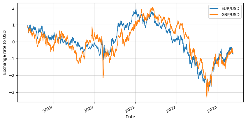
Example of multivariate data: Euro and Sterling Pound exchange range to US Dollars
VAR models are widely used for time series forecasting in finance, but this is not their only application, they are also used in many other domains. Some of their main applications include:
- Macroeconomic Forecasting: VAR models are commonly used in macroeconomic analysis to forecast key economic variables such as GDP growth, inflation rates, interest rates, exchange rates, and unemployment rates. They are able to consider the interdependencies among multiple economic variables, to capture complex interactions and provide accurate forecasts.
- Financial Market Analysis: VAR models are utilized in financial market analysis to forecast asset prices, volatility, and other financial variables. They can capture the dynamic relationships between different financial time series, to make predictions about future market movements and manage risk effectively.
- Energy Demand and Price Forecasting: VAR models are employed in forecasting energy demand and prices in the energy sector. They can take into account multiple factors that influence energy demand and prices, such as weather conditions, economic indicators, and supply-demand dynamics. These models help energy companies and policymakers make informed decisions about production, distribution, and pricing.
- Marketing and Sales Forecasting: VAR models can be employed in marketing and sales forecasting to predict consumer behaviour and demand patterns. They consider several marketing and economic variables, such as advertising expenditure, consumer sentiment, and macroeconomic indicators, to provide insights into future sales volumes, market share, and customer preferences.
- Supply Chain and Inventory Management: VAR models find applications in supply chain management to forecast demand patterns, optimize inventory levels, and plan production schedules. By analyzing the relationships between different variables in the supply chain, such as sales, inventory levels, and lead times, they can improve operational efficiency and reduce costs.
- Environmental and Climate Forecasting: VAR models are utilized in environmental and climate forecasting to predict variables like temperature, rainfall, air quality, and pollutant levels. They can help make informed decisions regarding environmental management, resource allocation, and climate change mitigation.
VAR models offer a flexible framework for time series forecasting that accounts for interdependencies among multiple variables, making them suitable for various applications.
The key advantage of VAR models is their ability to capture the joint behaviour of multiple variables, providing more comprehensive predictions compared to univariate AR models.
However, the additional capabilities of VAR models add complexity, affecting interpretability and parameter estimation, which becomes a computationally intensive task.
In conclusion, the extension from univariate AR models to multivariate VAR models is a significant step forward in time series analysis. VAR models, by considering interactions and dependencies among variables, offer a powerful tool for understanding and predicting complex systems in various fields such as economics, finance, and epidemiology.


0 Comments