In previous articles, we’ve introduced how to use XGBoost to forecast future time series data points. We did that with univariate data and also added additional or exogenous variables. However, one limitation is that XGBoost models are not capable of handling multivariate data. Before moving forward, let’s clarify what each term means.
Univariate vs. Multivariate
Imagine that a store uses past records of daily total sales to forecast future sales. The forecast is based solely on historical sales data, predicting future sales amounts based on patterns like seasonality or trends observed in the past. This corresponds to a univariate data scenario.
While the store still aims to forecast future daily sales, it now incorporates an exogenous variable like daily advertising spend into its forecasting model. The prediction of future sales is now not just based on past sales but also considers how changes in advertising spending could influence future sales, even though advertising spending itself is not being forecasted. This is therefore univariate data with exogenous variables.
Imagine now that the store is interested in forecasting multiple interrelated variables such as daily sales, customer footfall, and the number of items sold. The forecasting model uses the historical data of all these variables to make interconnected predictions, taking into account how each variable may affect the others in the future. For instance, the model might predict that an increase in customer footfall could lead to an increase in both total sales and the number of items sold. This is an example of multivariate data forecasting.
To sum up:
- Univariate Forecasting: This approach uses data collected on a single variable to predict future values of that same variable. The forecasting model relies solely on the historical values of the variable to estimate its future state.
- Univariate Forecasting with Exogenous Variables: This method uses data on one primary variable along with data on one or more other external variables that are believed to influence the primary variable. The forecast of the primary variable is informed by its own history as well as the historical values of these exogenous variables.
- Multivariate Forecasting: This type of forecasting uses data involving two or more variables to predict future values for each variable. The forecasting model considers the historical interrelationships and dependencies between the variables to make predictions.
Now that this is clear we can carry on with a multivariate model.
Multivariate model
This was a univariate example in which we predicted the price of one Forex pair (EUR/USD) by using exogenous variables like other pairs. But what if we wanted to use multiple pairs at once? That would be a multivariate problem.
XGBoost does not support multivariate models. We would need to train one model per pair. But instead of this, we could simply use a Neural Network.
Similarly to what we’ve done with the previous analyses, we also need to reframe our data to a supervised learning problem. However, we will do it in a slightly different way, since now we will have more than one target variable. Let’s take one week of returns for each currency pair:
df_supervised_multi = pd.DataFrame()

for pair in df_logret.columns:
    df_supervised_x = reframe_to_supervised(df_logret[pair],
                                            window_size=7,
                                            target=True,
                                            target_name=True)
    df_supervised_multi = pd.concat((df_supervised_multi, df_supervised_x), axis=1).dropna()
We also need to split the features from the target as we did before:
target_columns = [col for col in df_train_multi.columns if "target" in col]

X_train_multi = df_train_multi.drop(columns=target_columns)
y_train_multi = df_train_multi[target_columns]

X_test_multi = df_test_multi.drop(columns=target_columns)
y_test_multi = df_test_multi[target_columns]
Let’s import the required libraries to train the neural network using Keras:
from tensorflow.keras.models import Sequential
from tensorflow.keras.layers import Dense
We need to define the input and output size of our neural network, which will be 42 (7 timesteps times 6 currencies) and 6 (number of currencies) respectively:
input_dim = X_train_multi.shape[1]
output_dim = y_train_multi.shape[1]
Next, create a neural network model using Keras’ Sequential API. Here, we’ll use a simple feedforward neural network (also known as a multi-layer perception) with 4 layers and 128 neurons each.
# Initialize the model
model = Sequential()

# Add layers
model.add(Dense(128, input_dim=input_dim, activation='relu'))
model.add(Dense(128, activation='relu'))
model.add(Dense(128, activation='relu'))
model.add(Dense(128, activation='relu'))

# Output layer with 3 output variables
model.add(Dense(output_dim, activation='linear'))
Compile the model, specifying the optimizer, loss function, and metrics to track.
model.compile(optimizer='Adam', loss='mse', metrics=['mae'])
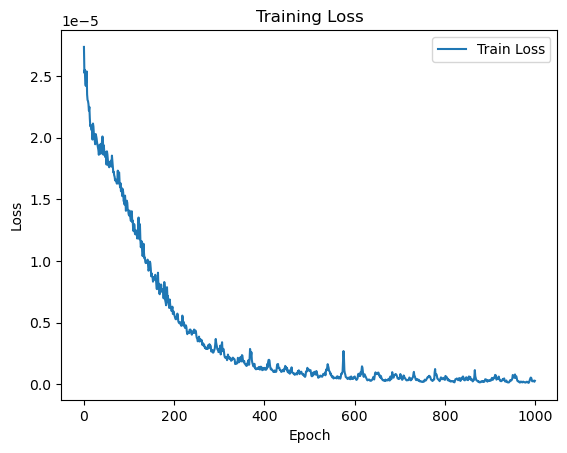
Let’s train it for 1000 epochs, with a batch size of 32.
history = model.fit(X_train_multi, y_train_multi,
                    epochs=1000, batch_size=32, verbose=1)
This is how the loss evolved during the 1000 epochs:
Time to forecast!
# Make predictions
predictions = model.predict(X_test_multi)

# Convert predictions to dataframe
df_predictions = pd.DataFrame(predictions, index=y_test_multi.index, columns=y_test_multi.columns)
Before plotting the predictions let’s address some issues with this approach.
Advanced functionalities of Keras
That way of training has several problems:
- We can’t visualise the evolution of the training loss
- If there is overfitting we can’t easily prevent it
- We can’t see if there is overfitting
That’s why we will implement some more advanced functionalities to have more control over our model.
Let’s first plot in real time the training loss. For that, we will define the following callback:
from tensorflow.keras.callbacks import Callback
from IPython.display import clear_output

class PlotLosses(Callback):
    def on_train_begin(self, logs={}):
        self.losses = []
        self.fig = plt.figure()
        self.logs = []

    def on_epoch_end(self, epoch, logs={}):
        self.logs.append(logs)
        self.losses.append(logs.get('loss'))

        clear_output(wait=True)
        plt.clf()  # Clear the current figure (prevents multiple plots)
        plt.plot(self.losses)
        plt.xlabel('Epoch')
        plt.ylabel('Loss')
        plt.title('Training Loss')
        plt.legend(['Train Loss'])
        plt.draw()
        plt.pause(0.001)
This will get the current loss and append it to a list of losses. After doing that it will clear the output and plot the losses. In this way, we can check how the training loss looks during training, and stop it manually to prevent the unnecessary use of resources.
This is how we add it to our model:
plot_losses = PlotLosses()

history = model.fit(X_train_multi,
                    y_train_multi,
                    epochs=1000,
                    batch_size=32,
                    verbose=1,
                    callbacks=[plot_losses])
We can also do it automatically, so it stops when the loss doesn’t improve for a particular number of epochs. This number of epochs is specified through the parameter patience. This strategy is called early stopping. We can define another callback to add it to our model.
from tensorflow.keras.callbacks import EarlyStopping

early_stopping = EarlyStopping(monitor='loss',
                               min_delta=0,
                               patience=10,
                               verbose=1,
                               mode='auto')
We can add it similarly to the previous callback:
history = model.fit(X_train_multi,
                    y_train_multi,
                    epochs=1000,
                    batch_size=32,
                    verbose=1,
                    callbacks=[plot_losses, early_stopping])
Finally, we would like to see how our model is performing. For this, we could plot the validation loss. This implies several modifications:
- We need to tell the model that we want a fraction of the data used as the validation set:
- We need to modify the PlotLosses callback so it plots the validation loss too.
- We need to change the loss that the EarlyStopping callback is tracking to the validation loss.
This is the resulting code:
# Callback for plotting losses
class PlotLosses(Callback):
    def on_train_begin(self, logs={}):
        self.epochs_loss = []
        self.epochs_val_loss = []
        self.fig = plt.figure()

    def on_epoch_end(self, epoch, logs={}):
        self.epochs_loss.append(logs.get('loss'))
        self.epochs_val_loss.append(logs.get('val_loss'))  # Capture validation loss
        clear_output(wait=True)
        plt.plot(self.epochs_loss, label='Training Loss')
        plt.plot(self.epochs_val_loss, label='Validation Loss')  # Plot validation loss
        plt.xlabel('Epoch')
        plt.ylabel('Loss')
        plt.title('Training and Validation Loss')
        plt.legend()
        plt.draw()
        plt.pause(0.001)

# Callback for early stopping
early_stopping = EarlyStopping(monitor='val_loss', patience=30, verbose=1, mode='min')

# Train the model
plot_losses = PlotLosses()
history = model.fit(X_train_multi, y_train_multi,
                    epochs=1000,
                    batch_size=32,
                    verbose=1,
                    callbacks=[plot_losses, early_stopping],
                    validation_split=0.2)  # 20% of the data will be used as a validation set
We’ve increased the patience to 30 epochs to prevent a too-early stopping. This is the resulting loss plot:
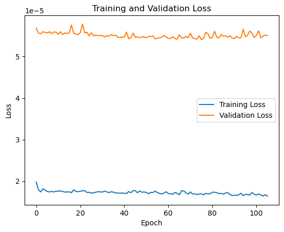
We can see that it makes no sense to keep training the model as the validation loss is not decreasing. This could lead to overfitting, therefore the early stopping callback stopped the training process.
Results
Time to predict and plot the results:
# Make predictions
predictions = model.predict(X_test_multi)

# Convert predictions to dataframe
df_predictions = pd.DataFrame(predictions, index=y_test_multi.index, columns=y_test_multi.columns)

# Plot predictions
for i, pair in enumerate(df_logret.columns):
    df_predictions.iloc[-30:,i].plot(figsize=(8,5))
    y_test_multi.iloc[-30:,i].plot()
    plt.legend(['Forecast', 'Actual'])
    plt.grid(alpha=0.3)
    plt.title(pair)
    plt.xlabel('Date')
    plt.ylabel('Log returns')
    plt.show()
For simplicity let’s plot the log returns of only two pairs:
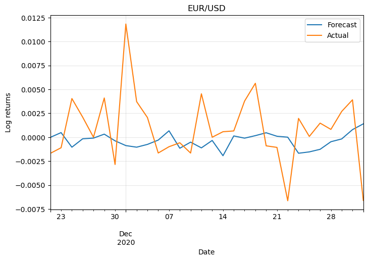
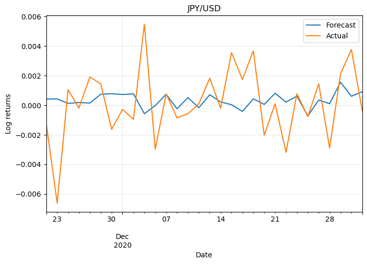
They don’t look promising. This is because the model wasn’t optimised and also because we need more information to make predictions. Also, Forex markets are unpredictable most of the time, otherwise, anyone could easily become rich!
Finally, let’s inspect the prices. We need to convert the log returns to prices first:
import datetime

for pair in df_logret.columns:
    # Get previous day's price
    prices_yesterday = df.loc[y_test_multi.index[0] - datetime.timedelta(1):, f'{pair}'].shift(1).dropna()

    # Forecasted prices
    y_pred_prices_multi = prices_yesterday * np.exp(df_predictions[f'target ({pair})'])

    plt.figure(figsize=(8,5))
    y_pred_prices_multi.iloc[-30:].plot()
    df.loc[y_test_multi.index, f'{pair}'].iloc[-30:].plot()
    plt.legend(['forecast', 'actual'])
    plt.xticks(rotation=45, ha='right')
    plt.grid(alpha=0.5)
    plt.ylabel('Prices')
    plt.legend(['Forecast', 'Actual'])
    plt.title(pair)
    plt.show()
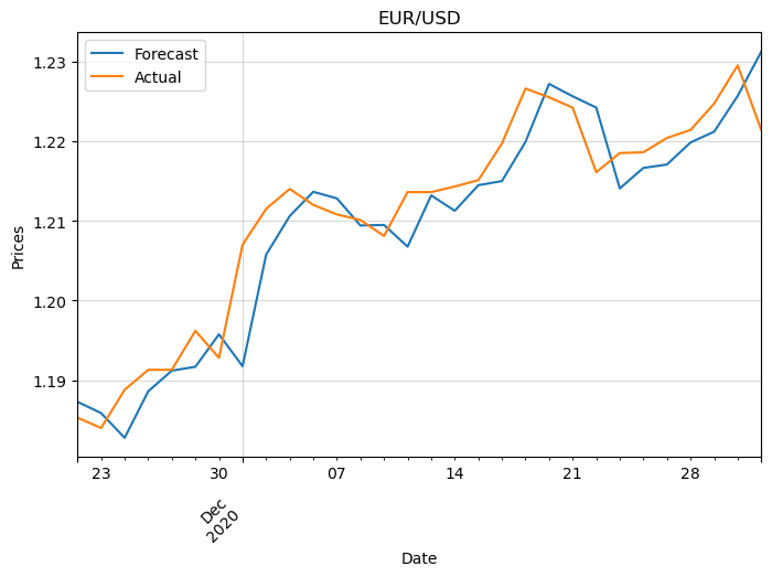
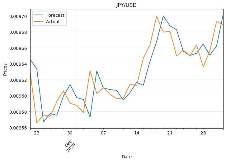
This confirms what we suspected with the log returns.


0 Comments