In a previous article, we introduced Vector Auto-Regression (VAR), a statistical model designed for multivariate time series analysis and forecasting. VAR provides a robust solution by effectively capturing dynamic relationships between multiple variables over time. In this article, we will train a VAR model step-by-step. We will use the dataset about the number of COVID cases and deaths in Germany, which we employed in the article we introduced Granger causality.
Data preparation
Let’s first import the basic libraries and the data. We will also convert the date to datetime, set it as index and keep only the values for dates and deaths. Finally, we will inspect the data visually.
# Import basic libraries for data analysis
import numpy as np
import pandas as pd
import matplotlib.pyplot as plt

# Read csv file
df_input = pd.read_csv('covid_de.csv')

# Convert the date column to datetime
df_input['date'] = pd.to_datetime(df_input.date, format='%Y-%m-%d')

# Group the data by day and keep only number of cases and deaths
df = df_input.groupby(['date']).sum()[['cases', 'deaths']]

# Visualise the data
df.plot()
plt.ylabel('Number of cases/deaths')
plt.show()
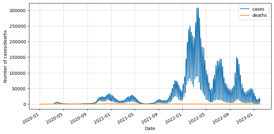
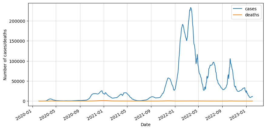
We can see that the data is really noisy because of the way the data was taken. Not every day the cases and deaths were recorded, so in order to minimize this effect we will do a 7-day rolling average.
# Apply a rolling average of 7 days
df_roll = df.rolling(7).mean().dropna()
# Plot results
df_roll.plot(figsize=(10,5))
plt.grid(alpha=0.5, which='both')
plt.xlabel('Date')
plt.ylabel('Number of cases/deaths')
plt.show()
The next step is to split it into training and testing sets. We will take 90% of the data for training. In this article we will only test the first 14 days of the testing set.
# Split into train and test
cutoff_index = int(df_roll.shape[0] * 0.9)
df_train = df_roll.iloc[:cutoff_index]
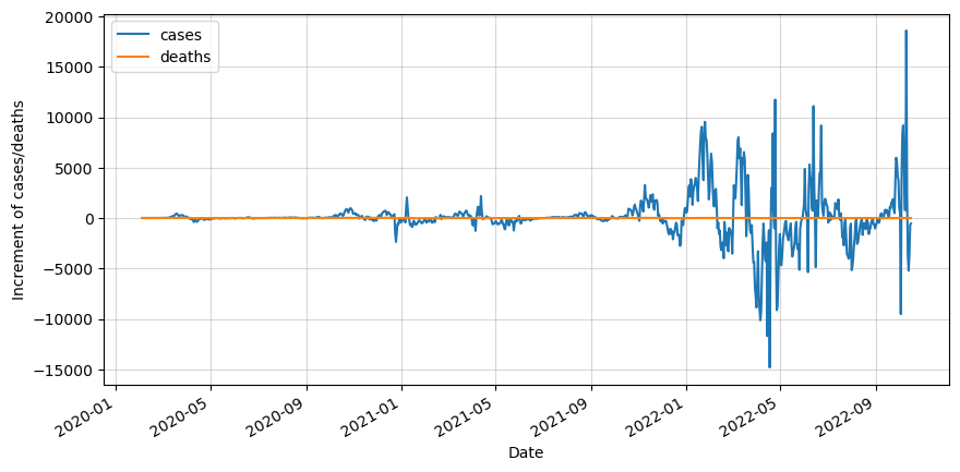
df_test = df_roll.iloc[cutoff_index:]We can clearly see that our data is not stationary. Therefore we will apply one differencing and test for stationarity.
# Apply differencing
df_diff = df_train.diff().dropna()

# Plot results
df_diff.plot(figsize=(10,5))
plt.grid(alpha=0.5, which='both')
plt.xlabel('Date')
plt.ylabel('Increment of cases/deaths')
plt.show()
Stay up-to-date with our latest articles!
Subscribe to our free newsletter by entering your email address below.
Now we check if one differencing is enough to make the data stationary.
from statsmodels.tsa.stattools import adfuller

for variable in df_diff.columns:

    # Perform the ADF test
    result = adfuller(df_diff[variable])

    # Extract and print the p-value from the test result
    p_value = result[1]
    print("p-value:", p_value)

    # Interpret the result
    if p_value <= 0.05:
        print(f"The variable {variable} is stationary.\n")
    else:
        print(f"The variable {variable} is not stationary.\n")
p-value: 1.6752374579302743e-09
The variable cases is stationary.
p-value: 0.0002010501151959319
The variable deaths is stationary.It was indeed sufficient.
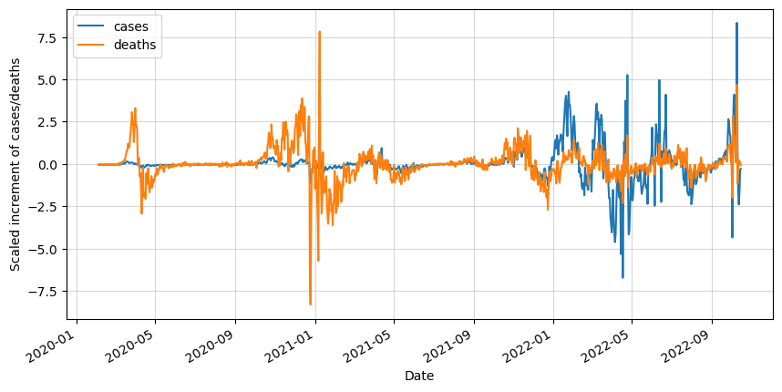
The following step is not strictly required, but it will help us visualize our data. We will proceed to scale it so we will be able to see how both variables compare to each other.
 # Import StandardScaler
from sklearn.preprocessing import StandardScaler

# Instantiate the scaler
scaler = StandardScaler()

# Transform data
scaled_values = scaler.fit_transform(df_diff)

# Convert to dataframe
df_scaled = pd.DataFrame(scaled_values,
                         columns=df_diff.columns,
                         index=df_diff.index)

# Visualize data
df_scaled.plot(figsize=(10,5))
plt.grid(alpha=0.5, which='both')
plt.xlabel('Date')
plt.ylabel('Scaled increment of cases/deaths')
plt.show()
It is good to do it step by step, but if you are planning to do the same in the future is it recommended to create a function that automatically performs all these steps.
In our case, we need to do it again with the testing set. We will define a function that processes the data. Because we are differencing, it is recommended to use the whole dataset and split it again into testing set within the function. Finally, use our function to generate the precessed testing set.
# Define function for data transformation
def df_test_transformation(df, test_start_date, scaler):

    # Apply differencing to make data stationary
    df_diff = df.diff().dropna()

    # Scale data using the previously defined scaler
    df_scaled = pd.DataFrame(scaler.fit_transform(df_diff),
                         columns=df_diff.columns,
                         index=df_diff.index)

    # Select only the data that belongs to the testing set
    df_test_processed = df_scaled[df_scaled.index > test_start_date]

    return df_test_processed

# Apply function to our data
df_test_processed = df_test_transformation(df_roll, df_scaled.index[-1], scaler)
After training the model we will generate predictions, however, they will be “processed” and we want them in the original scale and not differenced. That’s why we need to create a function that is able to bring the data back to the original format. We will call this to invert the transformations. Please note that one of the arguments is the original dataset, this is because after inverting the differencing with a cumulative summation, we need to add the actual value of the day before.
# Define function for inverting data transformation
def df_inv_transformation(df_processed, df, scaler):

    # Invert StandardScaler transformation
    df_diff = pd.DataFrame(scaler.inverse_transform(df_processed),
                                columns=df_processed.columns,
                                index=df_processed.index)

    # Invert differenting
    df_original = df_diff.cumsum() + df[df.index < df_diff.index[0]].iloc[-1]

    return df_original
We are getting closer to the model training stage. But first, it is worth checking if the variables are somehow related and will help in the forecast of each other. We can use the Granger causality test as we saw in a previous article.
# Import library
from statsmodels.tsa.stattools import grangercausalitytests

# Deaths as a Granger-cause
deaths_as_cause = grangercausalitytests(df_scaled[['cases', 'deaths']], 5)
Granger Causality
number of lags (no zero) 1
ssr based F test: F=0.0136 , p=0.9074 , df_denom=974, df_num=1
ssr based chi2 test: chi2=0.0136 , p=0.9072 , df=1
likelihood ratio test: chi2=0.0136 , p=0.9072 , df=1
parameter F test: F=0.0136 , p=0.9074 , df_denom=974, df_num=1
Granger Causality
number of lags (no zero) 2
ssr based F test: F=0.9209 , p=0.3985 , df_denom=971, df_num=2
ssr based chi2 test: chi2=1.8514 , p=0.3963 , df=2
likelihood ratio test: chi2=1.8496 , p=0.3966 , df=2
parameter F test: F=0.9209 , p=0.3985 , df_denom=971, df_num=2
Granger Causality
number of lags (no zero) 3
ssr based F test: F=0.1353 , p=0.9390 , df_denom=968, df_num=3
ssr based chi2 test: chi2=0.4088 , p=0.9384 , df=3
likelihood ratio test: chi2=0.4087 , p=0.9384 , df=3
parameter F test: F=0.1353 , p=0.9390 , df_denom=968, df_num=3
Granger Causality
number of lags (no zero) 4
ssr based F test: F=0.2274 , p=0.9231 , df_denom=965, df_num=4
ssr based chi2 test: chi2=0.9181 , p=0.9220 , df=4
likelihood ratio test: chi2=0.9177 , p=0.9220 , df=4
parameter F test: F=0.2274 , p=0.9231 , df_denom=965, df_num=4
Granger Causality
number of lags (no zero) 5
ssr based F test: F=0.1590 , p=0.9773 , df_denom=962, df_num=5
ssr based chi2 test: chi2=0.8039 , p=0.9768 , df=5
likelihood ratio test: chi2=0.8036 , p=0.9768 , df=5
parameter F test: F=0.1590 , p=0.9773 , df_denom=962, df_num=5
# Cases as a Granger-cause
cases_as_cause = grangercausalitytests(df_scaled[['deaths', 'cases']], 5)
Granger Causality
number of lags (no zero) 1
ssr based F test: F=3.9978 , p=0.0458 , df_denom=974, df_num=1
ssr based chi2 test: chi2=4.0101 , p=0.0452 , df=1
likelihood ratio test: chi2=4.0019 , p=0.0454 , df=1
parameter F test: F=3.9978 , p=0.0458 , df_denom=974, df_num=1
Granger Causality
number of lags (no zero) 2
ssr based F test: F=15.3471 , p=0.0000 , df_denom=971, df_num=2
ssr based chi2 test: chi2=30.8522 , p=0.0000 , df=2
likelihood ratio test: chi2=30.3746 , p=0.0000 , df=2
parameter F test: F=15.3471 , p=0.0000 , df_denom=971, df_num=2
Granger Causality
number of lags (no zero) 3
ssr based F test: F=10.1727 , p=0.0000 , df_denom=968, df_num=3
ssr based chi2 test: chi2=30.7389 , p=0.0000 , df=3
likelihood ratio test: chi2=30.2643 , p=0.0000 , df=3
parameter F test: F=10.1727 , p=0.0000 , df_denom=968, df_num=3
Granger Causality
number of lags (no zero) 4
ssr based F test: F=7.6732 , p=0.0000 , df_denom=965, df_num=4
ssr based chi2 test: chi2=30.9790 , p=0.0000 , df=4
likelihood ratio test: chi2=30.4966 , p=0.0000 , df=4
parameter F test: F=7.6732 , p=0.0000 , df_denom=965, df_num=4
Granger Causality
number of lags (no zero) 5
ssr based F test: F=5.3036 , p=0.0001 , df_denom=962, df_num=5
ssr based chi2 test: chi2=26.8211 , p=0.0001 , df=5
likelihood ratio test: chi2=26.4581 , p=0.0001 , df=5
parameter F test: F=5.3036 , p=0.0001 , df_denom=962, df_num=5
We see that the number of cases has the potential of improving the forecast of the number of deaths, as cases Granger-cause deaths. However, this doesn’t happen the other way around. It is therefore interesting to use a model that can use both variables to forecast the future. The simplest multivariate model we think of is the Vector Autoregression model or VAR.
Vector Autoregression
We will start by importing the VAR library and instantiating the model.
# Import library
from statsmodels.tsa.vector_ar.var_model import VAR

# Insantiate VAR model
model = VAR(df_scaled)
We need to find out what the optimal number of lags is. Statsmodels library makes this super easy with the select_order method.
# Get optimal lag order based on the four criteria
optimal_lags = model.select_order()

print(f"The optimal lag order selected: {optimal_lags.selected_orders}")
The optimal lag order selected: {'aic': 18, 'bic': 15, 'hqic': 16, 'fpe': 18}
We have 4 criteria available for the lag order selection:
- Akaike Information Criterion (AIC): AIC is a criterion that measures the goodness of fit of a statistical model while taking into account the model’s complexity. The goal is to minimize this value, so a lower AIC indicates a better-fitting model.
- Bayesian Information Criterion (BIC): BIC is similar to AIC but penalizes model complexity more heavily. It aims to strike a balance between model fit and complexity. Like AIC, the goal is to minimize the BIC value.
- Hannan-Quinn Information Criterion (HQIC): HQIC is another information criterion used for model selection in VAR models. It addresses the issue of small sample sizes by providing a different penalty term for model complexity. The goal is also to minimize this value.
- Final Prediction Error (FPE): FPE is a criterion used specifically for VAR models. It measures the mean squared error of the model’s one-step-ahead prediction. The goal is to minimize this value.
For the sake of simplicity and interpretability, we will keep the lowest optimal lag order, in this case, 8, corresponding to the BIC criterion.
We now train the model with the selected lag order and visualize the model summary.
# Fit the model after selecting the lag order
lag_order = optimal_lags.selected_orders['bic']
results = model.fit(lag_order)

# Estimate the model (VAR) and show summary
var_model = results.model
results.summary()
Summary of Regression Results
==================================
Model: VAR
Method: OLS
Date: Thu, 29, Jun, 2023
Time: 09:16:22
--------------------------------------------------------------------
No. of Equations: 2.00000 BIC: -1.48520
Nobs: 963.000 HQIC: -1.67936
Log likelihood: -1804.78 FPE: 0.165514
AIC: -1.79874 Det(Omega_mle): 0.155352
--------------------------------------------------------------------
Results for equation cases
=============================================================================
coefficient std. error t-stat prob
-----------------------------------------------------------------------------
const -0.002516 0.020988 -0.120 0.905
L1.cases 0.681215 0.035696 19.084 0.000
L1.deaths 0.016152 0.034570 0.467 0.640
L2.cases -0.158836 0.044333 -3.583 0.000
L2.deaths -0.001655 0.040875 -0.041 0.968
L3.cases 0.213803 0.045200 4.730 0.000
L3.deaths -0.015328 0.041684 -0.368 0.713
L4.cases -0.091696 0.045682 -2.007 0.045
L4.deaths 0.018695 0.041914 0.446 0.656
L5.cases 0.185565 0.045601 4.069 0.000
L5.deaths -0.015845 0.041907 -0.378 0.705
L6.cases 0.144317 0.045909 3.144 0.002
L6.deaths 0.051594 0.042027 1.228 0.220
L7.cases -0.455074 0.047490 -9.583 0.000
L7.deaths -0.048345 0.041935 -1.153 0.249
L8.cases 0.418564 0.048891 8.561 0.000
L8.deaths 0.024091 0.040730 0.591 0.554
L9.cases -0.160478 0.049685 -3.230 0.001
L9.deaths -0.021612 0.042141 -0.513 0.608
L10.cases 0.146508 0.049917 2.935 0.003
L10.deaths 0.000909 0.042453 0.021 0.983
L11.cases -0.125630 0.050104 -2.507 0.012
L11.deaths -0.025418 0.042376 -0.600 0.549
L12.cases 0.146269 0.049806 2.937 0.003
L12.deaths -0.010185 0.042426 -0.240 0.810
L13.cases 0.075932 0.049082 1.547 0.122
L13.deaths 0.000370 0.042281 0.009 0.993
L14.cases -0.110574 0.049197 -2.248 0.025
L14.deaths -0.063687 0.041409 -1.538 0.124
L15.cases -0.097255 0.039773 -2.445 0.014
L15.deaths 0.070984 0.034780 2.041 0.041
=============================================================================
Results for equation deaths
=============================================================================
coefficient std. error t-stat prob
-----------------------------------------------------------------------------
const -0.000799 0.021285 -0.038 0.970
L1.cases -0.140718 0.036201 -3.887 0.000
L1.deaths 0.694259 0.035059 19.802 0.000
L2.cases 0.143463 0.044960 3.191 0.001
L2.deaths -0.233079 0.041453 -5.623 0.000
L3.cases 0.005840 0.045840 0.127 0.899
L3.deaths 0.118811 0.042274 2.811 0.005
L4.cases -0.023814 0.046328 -0.514 0.607
L4.deaths 0.028070 0.042507 0.660 0.509
L5.cases -0.005836 0.046246 -0.126 0.900
L5.deaths 0.134878 0.042500 3.174 0.002
L6.cases 0.043507 0.046559 0.934 0.350
L6.deaths 0.181353 0.042621 4.255 0.000
L7.cases -0.065466 0.048162 -1.359 0.174
L7.deaths -0.258682 0.042529 -6.083 0.000
L8.cases 0.017050 0.049583 0.344 0.731
L8.deaths 0.391522 0.041306 9.479 0.000
L9.cases 0.035516 0.050388 0.705 0.481
L9.deaths -0.214305 0.042737 -5.014 0.000
L10.cases -0.011872 0.050623 -0.235 0.815
L10.deaths 0.126287 0.043053 2.933 0.003
L11.cases -0.010741 0.050813 -0.211 0.833
L11.deaths -0.043419 0.042975 -1.010 0.312
L12.cases 0.024729 0.050510 0.490 0.624
L12.deaths 0.001431 0.043026 0.033 0.973
L13.cases 0.053775 0.049777 1.080 0.280
L13.deaths 0.006112 0.042880 0.143 0.887
L14.cases 0.026710 0.049893 0.535 0.592
L14.deaths -0.326363 0.041995 -7.771 0.000
L15.cases -0.090187 0.040336 -2.236 0.025
L15.deaths 0.222209 0.035272 6.300 0.000
=============================================================================
Correlation matrix of residuals
cases deaths
cases 1.000000 0.399186
deaths 0.399186 1.000000
We can see that most of the p-values for the “equation cases” are below the significance level (0.05) for the cases lags, and above for the deaths lags. That can be interpreted as the number of deaths not contributing to the prediction.
However, on the “equation deaths” we can see low p-values for the deaths lags, and for specific cases lags also p-values below the significance level. So in this case the number of cases is helping forecast the number of deaths.
Let’s forecast the following 2 weeks of the number of cases and deaths. Note that it is required to input the last “lag_order” values from the training set in addition to the forecasting horizon of 14 days.
# Forecast next two weeks
horizon = 14
forecast = results.forecast(df_scaled.values[-lag_order:], steps=horizon)

# Convert to dataframe
df_forecast = pd.DataFrame(forecast,
                           columns=df_scaled.columns,
                           index=df_test.iloc[:horizon].index)
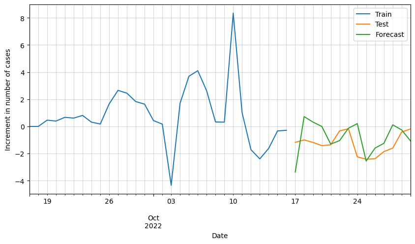
We can now visualise the results and compare them to the testing set.add Codeadd Markdown
# Plot forecasted increment of cases
ax = df_scaled[-30:].cases.plot(figsize=(10,5))
df_test_processed[:horizon].cases.plot(ax=ax)
df_forecast.cases.plot(ax=ax)
plt.grid(alpha=0.5, which='both')
plt.xlabel('Date')
plt.ylabel('Increment in number of cases')
plt.legend(['Train', 'Test', 'Forecast'])
plt.show()
# Plot forecasted increment of deaths
ax = df_scaled[-30:].deaths.plot(figsize=(10,5))
df_test_processed[:horizon].deaths.plot(ax=ax)
df_forecast.deaths.plot(ax=ax)
plt.grid(alpha=0.5, which='both')
plt.xlabel('Date')
plt.ylabel('Increment in number of deaths')
plt.legend(['Train', 'Test', 'Forecast'])
plt.show()
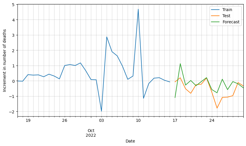
We can see that the results are pretty good, but it looks like there is room for improvement. Possibly by adding additional variables such as vaccinations, hospital occupation, etc., we could improve these results.
The last step is to bring the values back to the original data scale by applying the previously defined inverse transformation function.
# Invert the transformations to bring it back to the original scale
df_forecast_original = df_inv_transformation(df_forecast, df_roll, scaler)
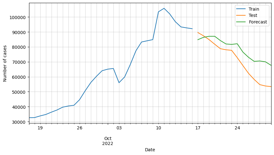
Let’s plot again the forecasts but this time in the original scale.
# Plot forecasted number of cases
ax = df_train[-30:].cases.plot(figsize=(10,5))
df_test[:horizon].cases.plot(ax=ax)
df_forecast_original.cases.plot(ax=ax)
plt.grid(alpha=0.5, which='both')
plt.xlabel('Date')
plt.ylabel('Number of cases')
plt.legend(['Train', 'Test', 'Forecast'])
plt.show()
# Plot forecasted number of deaths
ax = df_train[-30:].deaths.plot(figsize=(10,5))
df_test[:horizon].deaths.plot(ax=ax)
df_forecast_original.deaths.plot(ax=ax)
plt.grid(alpha=0.5, which='both')
plt.xlabel('Date')
plt.ylabel('Number of deaths')
plt.legend(['Train', 'Test', 'Forecast'])
plt.show()
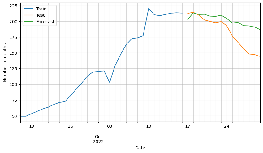
We can observe that the predictions are following the general trend, but as said before, there are some variables missing that must be affecting greatly the forecast.
This is proof of how useful multivariate models like VAR can be. Some models such as VARMA could also be used to improve the forecast, however, they are very difficult to optimize due to their high complexity.


0 Comments