XGBoost to forecast univariate Time Series data

In a previous article, we talked about the Advanced Time Series models. We mentioned that these are models based on Machine Learning. Some of the most common ones are based on Neural Networks, these are:

• Recursive Neural Networks or RNN
• Convolutional Neural Networks or CNN
• Transformers

These are great examples, but before moving to explain them, we should have a look at more straightforward ones. For example, based on more traditional Machine Learning models like Random Forest or XGBoost.

There is a particularity about this type of model, you will need to reframe the problem into a supervised learning one. We will introduce that here.

Import basic libraries and load data

We will import the basic libraries that we use in every single Data Science project, these are pandas, numpy and matplotlib.

import pandas as pd
import numpy as np
from matplotlib import pyplot as plt

Next, we load the data. In our case, we will load a dataset with Forex data with 3 years of records starting from 2018. This data includes six different currency prices with respect to the US Dollar (USD). These are also called Forex (Foreign Exchange) pairs. For this example, we will focus on the Euro to Dollar pair.

Let’s load the data and inspect it:

df = pd.read_csv('data.csv')

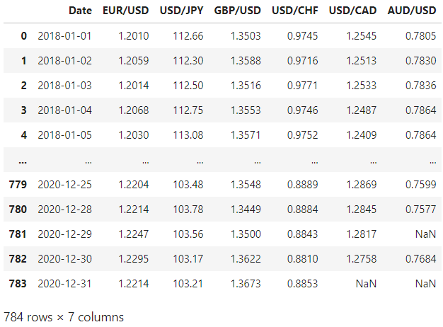
We observe some missing values, we can just fill them with the previous ones (forward fill) since it probably means that the Forex market was closed those days. Also, we notice that there are no values on the weekends, that’s because of the same reason, the Forex market is closed.

df = df.ffill()

Next, we need to convert the date column to datetime format and set it as the index.

# Convert date to datetime format
df['Date'] = pd.to_datetime(df['Date'], format='%Y-%m-%d')

# Set date as the index
df = df.set_index(['Date'])

Let’s also remove the pairs that we are not interested in including in our analysis. So we will retain only EUR/USD.

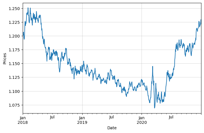
We can see that the price data is non-stationary.

Calculation of Log-Returns

So now we have the prices for the Euro with respect to the US Dollar. As you may have noticed already, non-stationary data is not the best one when working with Time Series data. This is the main reason why prices are not used in Finance. One possibility is using the difference between prices, but this only gives the absolute change and doesn’t provide information on the relative or percentage change. That is why log returns are widely used. But also, because of other two main reasons:

• Time Additivity: Log returns are time-additive. If you know the log returns of an asset for two consecutive periods, their sum gives the log return for the combined period. This property simplifies analyses and computations, especially in time series modelling.
• Statistical Properties: Log returns tend to be more normally distributed than simple returns, especially when returns are high. This normality assumption underpins many financial theories and models.

Using log returns simplifies mathematical modelling, makes time-series analysis more straightforward, and aligns with many statistical assumptions made in financial theories.

The formula for log returns, given the natural logarithm, is:

$$ r_t = \ln \left( \frac{P_t}{P_{t-1}} \right) $$

Where:

• $ r_t $ is the log return at time $ t $
• $ P_t $ is the price at time $ t $
• $ P_{t-1} $ is the price at the previous time period (time $ t-1 $)
• $ \ln $ denotes the natural logarithm.

Essentially, the log return is the natural logarithm of the ratio of the price at time $ t $ to the price at the previous time period.

Having said that, let’s proceed with their calculation:

df_logret = np.log(df).diff()
df_logret.dropna(inplace=True)

This is how the log returns look:

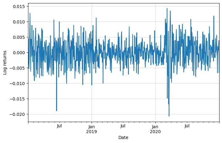
We can see that the data now resembles a stationary one, which is the desired type for this analysis.

Reframe to a Supervised Learning problem

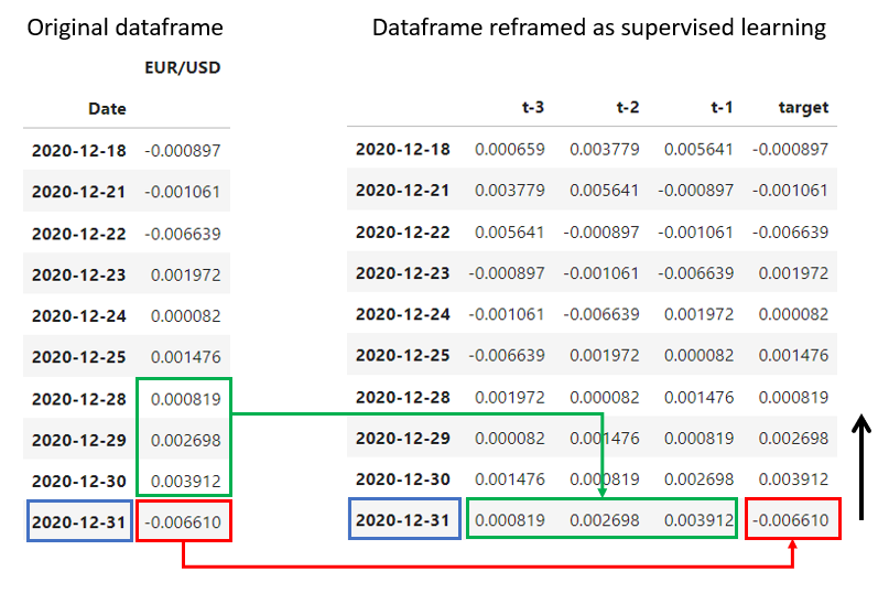
The idea here is to pass from a dataframe that has one column with the returns for each day (in addition to the date column or index), to a dataframe with multiple features (the X) and a target variable (the y).

We can achieve this simply by selecting a number of previous days to consider, let’s say 3 previous days, and create 3 features in that initial dataframe corresponding to the returns of the three previous days:

• Features: returns corresponding to $t-1$, $t-2$ and $t-3$.
• Target: returns corresponding to the time $t$.

This is achieved by moving a window through the dataset and relocating this data:

This is what we do with the following function. The window size will define the number of previous returns we will consider as features.

def reframe_to_supervised(df:pd.Series, window_size=7):
    # Initialize empty dataframe
    df_supervised = pd.DataFrame()

    # Define columns names
    X_columns = [f't-{window_size-i}' for i in range(window_size)]
    columns = X_columns + ['target']

    # Iterate
    for i in range(0, df.shape[0] - window_size):
        # Extract the last "window_size" observations and target
        # value and create an individual dataframe with this info
        df_supervised_i = pd.DataFrame([df.values[i:i+window_size+1]],
                                      columns=columns,
                                      index=[df.index[i+window_size]])

        # Add to the final dataframe
        df_supervised = pd.concat((df_supervised, df_supervised_i),
                                   axis=0)

    return df_supervised

Let’s use a window of 7 days, a week

df_supervised = reframe_to_supervised(df_logret['EUR/USD'], window_size=7)

Done! We now have a dataframe suitable for one of the Machine Learning models that we typically use in a supervised regression problem.

Before training our model we need to split into training and testing:

# Define the proportion of samples that will be added to the training set
training_proportion = 0.80

# We can calculate how many samples correspond to that proportion
n_obs = df_supervised.shape[0]
n_train = int(n_obs * training_proportion)

We are in a Time Series problem, which means that we cannot randomly split the data, we need to select one set from the beginning as a training set and one from the end as a testing set. Having calculated how many samples we need to get for the training set, we can do the following to split our data:

# Training set
df_train = df_supervised.iloc[:n_train]

# Testing set
df_test = df_supervised.iloc[n_train:]

We also need to split the features from the target

# Training set
X_train = df_train.drop(columns=['target'])
y_train = df_train['target']

# Testing set
X_test = df_test.drop(columns=['target'])
y_test = df_test['target']

Model training

Time to train our model. We will use first a simple Linear Regression model.

Linear Regression

We will train the most basic model to see how it behaves.

from sklearn.linear_model import LinearRegression
from sklearn.metrics import mean_squared_error

# Initialize the Linear Regression model
regressor = LinearRegression()

# Train the model using the training data
regressor.fit(X_train, y_train)

# Predict the outputs for the test data
y_pred = regressor.predict(X_test)

# Calculate and print the RMSE
rmse = mean_squared_error(y_test, y_pred, squared=False)
print(f"RMSE: {rmse}")

RMSE: 0.0039683982364106096

We get a pretty low RMSE, let’s see how the prediction is. As a note, we use the previous week of prices to predict the current price.

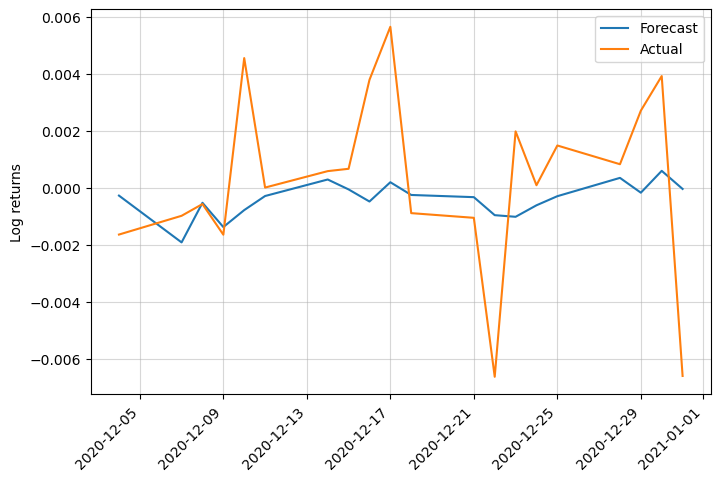
Despite a low RMSE, the predictions are not great.

Let’s try with a more complex and powerful model: XGBoost

XGBoost

First, if you don’t have it already, you will need to install XGBoost.

!pip install xgboost

The next steps are:

• import the library
• convert dataframes into DMatrix format, which is a data structure unique to XGBoost
• set XGBoost parameters for regression and number of boosting rounds

Finally, we can train the model and predict the values.

import xgboost as xgb

# Convert the datasets into DMatrix
dtrain = xgb.DMatrix(X_train, label=y_train)
dtest = xgb.DMatrix(X_test)

# Set XGBoost parameters
param = {
    'max_depth': 3,
    'eta': 0.3,
    'objective': 'reg:squarederror'
}

# Number of boosting rounds
num_round = 100

# Train the model
bst = xgb.train(param, dtrain, num_round)

# Predict the target for the test set
y_pred = bst.predict(dtest)

# Calculate and print the RMSE
rmse = mean_squared_error(y_test, y_pred, squared=False)
print(f"RMSE: {rmse}")

RMSE: 0.004409998153454305

Let’s visualize the prediction:

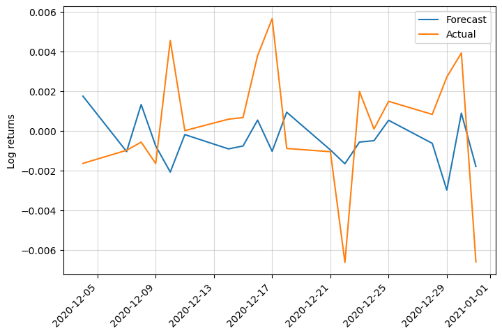
We can see that XGBoost is more responsive but the predictions are not better…

Visualizing prices

So far we have worked with the log returns, but we want to see how the prices behave. We need to invert the changes made.

This is the formula we will use:

$$ \text{Price}_{t} = \text{Price}_{t-1} \times e^{\text{Log Return}_{t}} $$

import datetime

# Get previous day's price
prices_yesterday = df.loc[y_test.index[0] - datetime.timedelta(1): ,'EUR/USD'].shift(1).dropna()

# Linear regression forecasted prices
y_pred_prices_lr = prices_yesterday * np.exp(y_pred_lr.forecast)

# XGBoost forecasted prices
y_pred_prices_xgb = prices_yesterday * np.exp(y_pred_xgb.forecast)

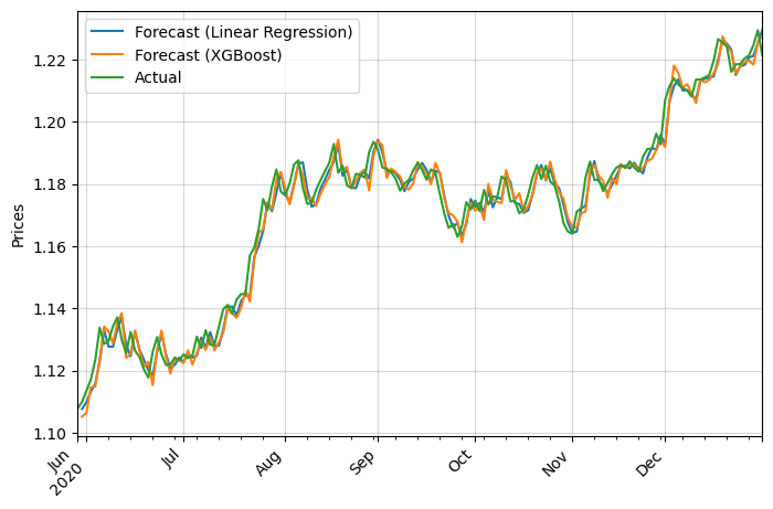
It looks alright. Let’s zoom in to appreciate it better:

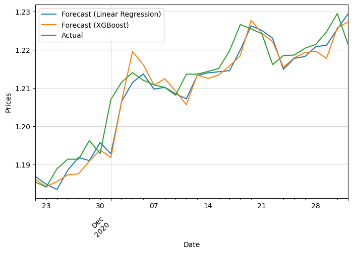
We can see that it is not great, as it seems like both of them are just replicating the last price with minimal adjustment. We should add more information with additional features:

• Day of the week and month
• Mean return during a certain period
• Technical indications such as Moving Average
• Exogenous variables like other Forex pairs

Let’s see how it improves just by adding some of them:

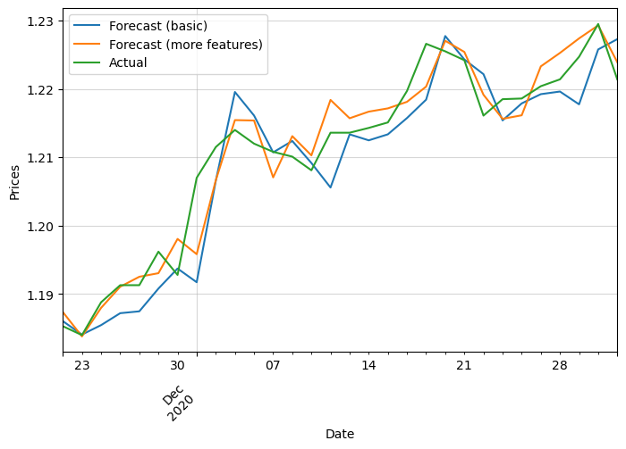
We can see that the new forecast manages to capture better the actual prices. It stays closer to it plus it’s able to predict some of the changing points. These are the features we added:

• month and day of week
• if price is above or below the 5, 10, 20 and 50 EMA and SMA
• mean during the last 7 days

The results considerably improve. We pass from an RMSE of 0.0044 to 0.0028!

Next time we will share the code to achieve this, in addition to adding more complex technical indicators and other Forex pairs. We will see what is the accuracy we can achieve!