Regularization

When training a Machine Learning model several scenarios can occur:

• The model can overfit, which means that the model is learning too much about the training data, it is too complex and it pays attention to very specific or random patterns within it or also called noise. This is a problem because the model won’t perform well on the testing data or real data.
• The model can underfit, which means that it is too simple, and not flexible enough. Therefore, it cannot learn all the relevant patterns within the data.
• The model is not too complex or too simple, it is able to find the relevant patterns within the data, without considering particular patterns in the training data. This is the ideal scenario and the one we will want for our model.

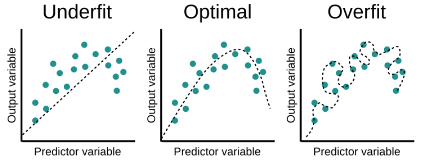
Model fitting scenarios. Source: educative.io

There are different techniques to identify which scenario we are in and how to achieve an optimal model in terms of complexity. One of the approaches is regularization.

Let’s first consider the Multiple Linear Regression formula:

$$ y^{(i)} = B_0 + B_1 x_1^{(i)} + … + B_n x_n^{(i)} $$

It is worth mentioning that each of the B coefficients determines the contribution of a feature in our data. Therefore, our data will have n different features. The index i refers to a particular datapoint in our dataset.

In Linear Regression, the optimization or loss function is the residual sum of squares:

$$\mathrm{J} = \sum_{n=1}^{n} (y^{(i)}-\hat y^{(i)})^2 = $$

$$ = \sum_{i=1}^{n} (y^{(i)}- B_0 – B_1 x_1^{(i)} – … – B_n x_n^{(i)})^2 $$

The model will be trained by estimating the B coefficients in a way that minimizes this function. If the training data contains noise, the coefficients won’t generalize well and the model won’t be able to properly predict future data.

Regularization

Regularization reduces the effect of noise in our model. It reduces the weight of those coefficients associated with noise, hence reducing their contribution to the prediction. For Linear Regression, this is achieved by constraining or shrinking the coefficients estimates towards zero, resulting in a simpler and less flexible model to prevent overfitting.

There are different regularization techniques, but we will cover the main two for Linear Regression:

Ridge Regression

In statistics, it is known as the L-2 norm. This technique consists of adding a small amount of bias to our model with the objective of improving the predictions. We can achieve this by adding the penalty or shrinkage term, which is the hyperparameter λ multiplied by the sum of the squared weight of each individual feature.

The optimization or loss function becomes:

$$\mathrm{J}_{Ridge} = \mathrm{J} + \lambda (B_1^2 + … + B_n^2) $$

λ controls how much regularization we want to apply to our model. It is selected in a process called hyperparameter tuning. If λ is set to zero, the optimization function becomes the one for Linear Regression.

On the one hand, Ridge regression can help when we have high collinearity between features. Also, it is useful when we have more features than samples.

On the other hand, this regularization technique shrinks the coefficients but never makes them zero, therefore it is not suitable for feature selection. Also, it does not help with the interpretability of the model, as it does not reduce the number of independent variables, only reduces their contribution.

In Python, it can be used through the scikit-learn library sklearn.linear_model.Ridge.

Lasso Regression

This regularization technique is known in statistics as the L-1 norm. It stands for Least Absolute and Selection Operator. Similarly to what we discussed in Ridge Regression, Lasso Regression includes a penalty term, which consists of the hyperparameter λ multiplied by the sum of the absolute weight of each individual feature.

The optimization or loss function becomes:

$$\mathrm{J}_{Lasso} = \mathrm{J} + \lambda (|B_1| + … + |B_n|) $$

Lasso Regression can force some of the coefficients to be exactly equal to zero. Therefore, this regularization technique is useful to do feature selection.

It has some limitations, for example, if the dataset is smaller than the number of features, Lasso Regression will consider only as many coefficients as the number of samples, leading to the possibility of ignoring some relevant coefficients. It also has problems with the interpretability of the model, as in the case of having highly correlated features, Lasso Regression will select one of them randomly.

Similarly to Ridge Regression, Lasso Regression can be used in Python through the scikit-learn library sklearn.linear_model.Lasso.

This was an introduction to the main two regularization techniques in Linear Regression. In future articles, we will deal with the mathematical side of it and why Lasso removes the contribution of certain features, whereas Ridge only diminishes their contribution.