Theoretical Introduction to Recurrent Neural Networks

Are you interested in mastering Time Series forecasting or natural language processing? Then you should learn about Recurrent Neural Networks.

Recurrent Neural Networks or RNNs are a specialized form of neural network architecture engineered for sequence-based tasks. Unlike traditional feed-forward neural networks, which treat each input as independent, RNNs excel in situations where the sequence and context are crucial.

The main difference with feed-forward neural networks is the “self-loop” they have in their neurons. In a “folded” RNN diagram, you’ll typically see neurons or units connected in a sequence where each neuron receives input and then passes its output (known as the hidden state) to the next neuron in line. This is unlike traditional neural networks where neurons pass information only in one direction: from the input layer to the output layer.

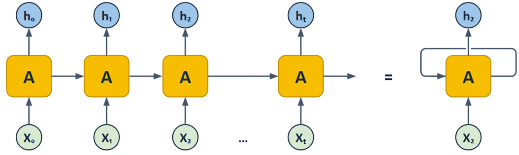
The “self-loop” in RNNs is represented by this hidden state being passed along from one step to the next in the sequence, helping it make a better decision based on what it knows from the past.

This self-loop allows the network to remember previous information and use it to inform later steps, creating an internal “memory” that helps in processing sequences. This is crucial for tasks like time-series forecasting or natural language understanding, where the order and context of data points matter.

RNN unit architecture

RNNs operate on a straightforward but powerful principle: each neuron in the network not only processes the current input but also incorporates a “memory” — often referred to as the “hidden state” — from previous steps. This hidden state allows the network to maintain contextual information over time, making RNNs perfect for tasks where understanding sequence and time is essential.

Let’s see how a basic or vanilla RNN unit is made of:

The RNN computes the hidden state $h_t$ as a function of the current input $x_t$ and the previous hidden state $h_{t-1}$. But, what exactly is each of these elements?

• Current Input ($x_t$): This is the data introduced into the model for each time step. It can be a word in a sentence or a data point in a time series.
• Previous Hidden State ($h_{t-1}$): This variable captures the network’s “memory” up to the prior time step. It contains essential historical information, serving as a contextual guide for the model’s current operations.
• New Hidden State ($h_{t}$): This updated hidden state emerges from the calculated combination of $x_t$ and $h_{t-1}$, factoring in the weight matrices. It serves as both the output for the current time step and the new “memory” ($h_{t-1}$) for subsequent steps.

Let’s see how these elements are related:

$$h_t = f(W_x · x_t + W_h · h_{t-1} + b)$$

We can distinguish several elements in this formula:

• Weight Matrices ($W_x$, $W_h$): These are learned parameters that dictate how much importance to give to the current input and the previous hidden state. They are critical for adjusting the impact of both the input and memory on the model’s decisions.
• Bias Term ($b$): Another learned parameter, the bias term fine-tunes the activation function, enabling the model to better fit the task’s specific data distribution.
• Activation Function ($f$): Functions like tanh or ReLU are used here to introduce non-linearity, enabling the model to capture more complex patterns in the data.

Utilizing the weight matrices ($W_x$, $W_h$), the RNN integrates the current input ($x_t$) and the previous hidden state ($h_{t-1}$) to generate a new hidden state ($h_{t}$). This process effectively combines current data with historical context. After generating $h_{t}$, this new hidden state is carried over to the next time step, becoming the new $h_{t-1}$ for future operations.

In essence, the RNN equation formalizes the process of updating the hidden state $h_{t}$ by incorporating both the current input $x_{t}$​ and the previous hidden state $h_{t-1}$​, thereby effectively utilizing both current and past information for sequence-based tasks.

This looped architecture allows RNNs to “remember” previous inputs, making them excellent for time series forecasting, natural language understanding, and any task requiring an understanding of underlying sequences.

Advantages and Disadvantages of RNNs

We have seen that RNNs are very cleverly designed. Therefore they have multiple advantages, but they also have disadvantages, especially when compared to their more advanced versions: LSTMs and GRUs:

Advantages

• Sequence Modeling: RNNs excel at handling sequences, which is crucial for tasks like time-series forecasting. For instance, they can predict stock prices by analyzing historical price data in sequence.
• Variable-Length Sequences: Unlike traditional neural networks that require a fixed-size input, RNNs can handle sequences of variable lengths. This is particularly beneficial for tasks like natural language processing where sentence lengths can vary widely.
• Parameter Sharing: RNNs have an architectural advantage as the same set of weights is used across all time steps. This not only reduces the model’s complexity but also facilitates faster and more efficient training, as fewer parameters generally make optimization easier.
• Context Awareness: Because RNNs maintain a hidden state, they can incorporate context when processing a sequence, which is essential for many natural language tasks. This is also particularly useful for time series with seasonality or other forms of dependency.
• Simpler Architecture: Compared to some other types of neural networks designed for sequence data, like LSTMs and GRUs, basic RNNs have a simpler architecture. This can make them easier to implement and quicker to train, although at the cost of some capabilities.
• Real-Time Processing: RNNs are designed to work with sequences and can process data in a streaming fashion. This makes them highly suitable for real-time applications such as financial trading, sensor data monitoring, and live speech-to-text conversion.
• Efficient Use of Memory: Due to parameter sharing across time steps, RNNs are relatively memory-efficient compared to models that do not share parameters. This can be an essential factor when deploying models to devices with limited memory resources.
• End-to-End Training: RNNs can be trained end-to-end, meaning that with enough data and computational resources, they can learn to map inputs to outputs without manual feature engineering. This is beneficial for tasks where it’s challenging to create effective features.

Disadvantages

• Vanishing/Exploding Gradients: Due to their architecture, RNNs are susceptible to vanishing and exploding gradient problems, which make them difficult to train on long sequences.
• Short-Term Memory: Basic RNNs have a limited “memory” and can find it difficult to learn long-term dependencies in the data.
• Computational Intensity: RNNs can be computationally intensive to train, especially for long sequences, which often makes them slower than other kinds of neural networks.
• Difficulty in Parallelization: Unlike feedforward neural networks, the recurrent nature of RNNs makes it difficult to parallelize the training process, leading to longer training times.
• Overfitting: RNNs can easily overfit the training data, especially when the dataset is small or not diverse enough.
• Interpreting Hidden State: The hidden state in an RNN captures information from all previous steps, but this can make it hard to interpret what the network is focusing on at any given time.
• Bias in Long Sequences: The architecture tends to give more weight to recent inputs in the sequence, potentially ignoring important information from earlier in the sequence.

Some of these disadvantages are addressed by LSTMs and GRUs, which are the types of Recurrent Neural Networks that we will see in future articles.