Step-by-Step Guide to Time Series Forecasting with Vanilla RNN

In the last article, we introduced the theory behind Recurrent Neural Networks. This time we will use a simple example to illustrate the process of training a vanilla or basic RNNs to forecast time series data.

We will import the basic libraries that we use in every single Data Science project, these are pandas, numpy and matplotlib.

import pandas as pd
import numpy as np
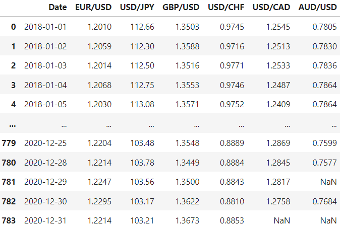
from matplotlib import pyplot as plt

Next, we load the data. We will use the same dataset as in the previous articles to be able to make a comparison. This is a dataset with Forex data with 3 years of records starting from 2018. This data includes six different currency prices with respect to the US Dollar (USD). These are also called Forex (Foreign Exchange) pairs. For this example, we will focus on forecasting the Euro to Dollar pair.

Let’s load the data and inspect it:

df = pd.read_csv('data.csv')

We need to address the missing values and the format of the date.

# Fill missing values
df = df.ffill()

# Convert date to datetime format
df['Date'] = pd.to_datetime(df['Date'], format='%Y-%m-%d')

# Set date as the index
df = df.set_index(['Date'])

We want all of the different currencies referenced to US Dollars, that’s why we need to apply the inverse if that’s not the case:

for pair in df.columns:
    if (pair.split('/')[0] == 'USD') & (pair.split('/')[1] != 'USD'):
        df[f"{pair.split('/')[1]}/{pair.split('/')[0]}"] = 1 / df[pair]
        df = df.drop(columns=[pair])

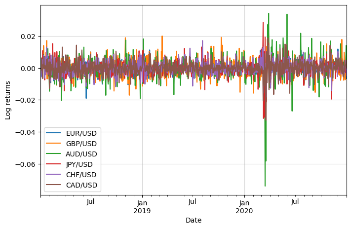
Let’s also calculate the log returns to make them stationary and bring them to a similar scale:

df_logret = np.log(df).diff()
df_logret.dropna(inplace=True)

Univariate

The next step is to reframe the dataset as a supervised problem. This time let’s work with numpy instead of using pandas.

We will focus for now only on the univariate problem, in other words, predicting the EUR/USD return using solely the previous returns. First, let’s convert our dataframe into a numpy array:

rets = df_logret['EUR/USD'].values

We will use the returns during the previous week (7 days) to predict the next day’s return.

# Initialize empty lists
x = []
y = []

# Set the wanted timesteps
timesteps = 7

# Iterate to populate the lists
for i in range(rets.shape[0] - timesteps):
    x.append(rets[i: i + timesteps])
    y.append(rets[i + timesteps])

# Convert lists to numpy arrays    
x = np.array(x)
y = np.array(y)

Neural Networks employ a unique input structure that sets them apart from other Machine Learning algorithms. Rather than using pandas dataframes, they necessitate the use of numpy arrays. Specifically, for Recurrent Neural Networks (RNNs), the dimensions of the input and output variables must conform to the following guidelines:

• Independent Variables (X): The input tensor should have a three-dimensional shape, represented as: [number of samples, number of timesteps, number of features].
• Dependent Variable (y): The shape of the output tensor can vary depending on the task at hand. For simpler tasks like classification or regression, it is often a two-dimensional array with dimensions [number of samples, output features].

This ensures that the data is properly formatted for processing within the RNN architecture.

In our case,

• X: [776, 7, 1]
• y: [776, 1]

However, they don’t respect this structure:

x.shape, y.shape

((776, 7), (776,))

We need to reshape them:

x = x.reshape(*x.shape,1)
y = y.reshape(-1,1)

x.shape, y.shape

((776, 7, 1), (776, 1))

Now they have the right shape!

The next step is to split the data into training and testing sets. Let’s select 90% of the data for training and 10% for testing the model performance.

n_train = int(x.shape[0] * 0.9)
n_train

698

This corresponds to approximately the first 698 rows.

Train the RNN model

First, we need to import the required libraries:

import keras
from keras import layers

Let’s build the model and compile it. We will use a single vanilla RNN layer. It is important to define the number of units, the input shape and the activation function.

We will use a tanh activation function. The tanh activation function is commonly used in RNNs for the following key reasons:

• Non-linearity: Enables the network to learn complex patterns.
• Output Range: Output values between −1 and 1, helping to centre the data.
• Vanishing Gradient: Mitigates the vanishing gradient problem to some extent.
• Gradient: Steeper gradient compared to sigmoid, aiding faster learning.

Setting the number of units (also known as neurons or hidden states) in an RNN is more of an art than an exact science, but there are some general guidelines you can follow:

• Experimentation: The most reliable way to determine the optimal number of units is through experimentation. You can use techniques like cross-validation to evaluate different configurations.
• Problem Complexity: For simple tasks, a smaller number of units may be sufficient. For more complex tasks involving long sequences, you may need more units to capture the complexity.
• Computational Resources: More units generally require more computational resources. Make sure your choice aligns with the hardware you have available.
• Overfitting vs. Underfitting: A large number of units may lead to overfitting, especially if you have limited data. Also, too few units may result in underfitting. Regularization techniques can help balance this.
• Architecture: The number of units often depends on the specific RNN architecture you’re using. For example, LSTMs and GRUs might require different numbers of units compared to vanilla RNNs.
• Empirical Rules: Some practitioners follow empirical rules, like setting the number of units to be somewhere between the size of the input layer and the size of the output layer.
• Grid Search: Automated hyperparameter tuning methods like grid search or random search can help you find an optimal number of units.

We will set it to 5 to start with. This is something that we could optimize as previously said.

The input shape is the number of timesteps by the number of features, in this case [7, 1].

# Initialize the Sequential model
model = keras.Sequential()

# Add an RNN layer with 5 units and tanh activation
model.add(layers.SimpleRNN(5, 
                           activation='tanh', 
                           use_bias=True, 
                           input_shape=(x.shape[1], x.shape[2])))

We can add a dropout layer. This serves primarily to combat overfitting. Here are the key reasons:

• Regularization: Dropout acts as a form of regularization by randomly setting a fraction of input units to 0 during training, which helps to prevent overfitting.
• Generalization: By deactivating some neurons during training, dropout forces the network to learn more robust features that generalize better to unseen data.
• Simplification: Dropout effectively creates a simpler model during each training iteration, reducing the model’s complexity.
• Ensemble Effect: Dropout can be seen as training a collection of sub-networks that share weights, contributing to a sort of ensemble effect, which often results in better performance.

Adding dropout layers is a common practice but should be done carefully to avoid underfitting or extended training times. Typical dropout rates are between 0.2 and 0.5. We will set it to the lowest recommended value: 0.2.

# Add a Dropout layer with a rate of 0.2 to prevent overfitting
model.add(layers.Dropout(rate=0.2))

We could also add a Dense Layer, but this is not necessary. When should we use it?

We could use a Dense Layer if:

• Output Size: You need to transform the RNN output to a single value.
• Complexity: The RNN alone isn’t capturing stock price patterns well.
• Fine-tuning: You want extra parameters to improve performance.

We should skip Dense Layer if:

• Simplicity: The RNN is already effective.
• Overfitting: You have a small or noisy dataset.
• Computational Cost: You want to minimize training time.

Let’s include it just to make a more general model:

# Add a Dense layer with 1 unit for the output
model.add(layers.Dense(1))

Time to compile the model. We will use the MSE loss and the Adam optimizer:

# Compile the model with mean squared error loss function and adam optimizer
model.compile(loss='mean_squared_error', optimizer='adam')

Let’s see the architecture of our model:

# Display the architecture of the model
model.summary()

Model: "sequential"
_________________________________________________________________
 Layer (type)                Output Shape              Param #   
=================================================================
 simple_rnn (SimpleRNN)      (None, 5)                 35        
 dropout (Dropout)           (None, 5)                 0         
 dense (Dense)               (None, 1)                 6         
=================================================================
Total params: 41
Trainable params: 41
Non-trainable params: 0

Time to train it. As we said before, we will use only the first 90% of our data, corresponding to our training set. Since this is a Time Series problem, we must not shuffle the data. We will set the validation split to 20%, this reserves that percentage of the training data for validation purposes. The model will set this fraction of the training data aside and not use it for training. It will evaluate the validation loss and any validation metrics on this data at the end of each epoch.

# Fitting the data
history = model.fit(x[:n_train],
                    y[:n_train],
                    shuffle = False,
                    epochs=100,
                    batch_size=32,
                    validation_split=0.2,
                    verbose=1)

Epoch 1/100
18/18 [==============================] - 2s 23ms/step - loss: 1.0273e-04 - val_loss: 1.2418e-04
Epoch 2/100
18/18 [==============================] - 0s 6ms/step - loss: 7.6808e-05 - val_loss: 9.0449e-05
[...]
Epoch 99/100
18/18 [==============================] - 0s 6ms/step - loss: 1.5610e-05 - val_loss: 2.9889e-05
Epoch 100/100
18/18 [==============================] - 0s 6ms/step - loss: 1.5449e-05 - val_loss: 2.9902e-05

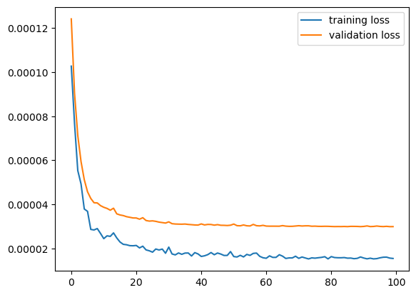
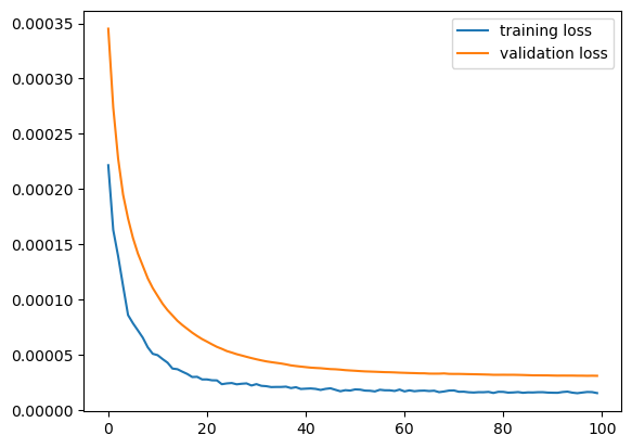
That output helps us see the evolution of the loss, however, viewing it in a graph always helps, let’s do that then:

# Plotting the loss iteration
plt.plot(history.history['loss'], label = 'training loss')
plt.plot(history.history['val_loss'], label ='validation loss')
plt.legend()
plt.show()

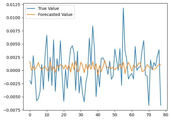
Let’s make the predictions:

y_true = y[n_train:]
y_pred = model.predict(x[n_train:])

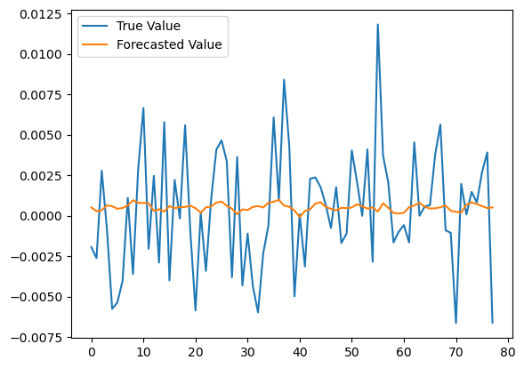
Let’s assess its performance by computing the Root Mean Squared Error (RMSE):

from sklearn.metrics import mean_squared_error
np.sqrt(mean_squared_error(y_true, y_pred))

0.0036406275418344263

We can see that the model is not good enough in predicting the returns. We need more data and more features to improve it. We could add the other currency pairs to see if there is an improvement.

Multivariate Single-output

The multivariate single-output process is very similar to the univariate, with few changes. We will go faster this time.

# Get returns for all pairs
rets_multi = df_logret.values

# Reframe to supervised problem
x_multi = []
y_multi = []
timesteps = 7

for i in range(rets_multi.shape[0] - timesteps):
    x_multi.append(rets_multi[i: i + timesteps])
    y_multi.append(rets_multi[i + timesteps][0])
      
x_multi = np.array(x_multi)
y_multi = np.array(y_multi)

# Check shape
x_multi.shape, y_multi.shape

((776, 7, 6), (776,))

This time the shape is correct from the beginning, so we don’t need further processing.

Train the multivariate RNN model

# Initialize the Sequential model
model = keras.Sequential()

# Add an RNN layer with 5 units and tanh activation
model.add(layers.SimpleRNN(5, activation='tanh', use_bias=True, input_shape=(x_multi.shape[1], x_multi.shape[2])))

# Add a Dropout layer with a rate of 0.2 to prevent overfitting
model.add(layers.Dropout(rate=0.2))

# Add a Dense layer with 1 unit for the output
model.add(layers.Dense(1))

# Compile the model with mean squared error loss function and adam optimizer
model.compile(loss='mean_squared_error', optimizer='adam')

# Display the architecture of the model
model.summary()

Model: "sequential_1"
_________________________________________________________________
 Layer (type)                Output Shape              Param #   
=================================================================
 simple_rnn_1 (SimpleRNN)    (None, 5)                 60        
 dropout_1 (Dropout)         (None, 5)                 0         
 dense_1 (Dense)             (None, 1)                 6         
=================================================================
Total params: 66
Trainable params: 66
Non-trainable params: 0

We fit the data in the same way as we did before:

# Fitting the data
history = model.fit(x_multi[:n_train],
                    y_multi[:n_train],
                    shuffle = False,
                    epochs=100,
                    batch_size=32,
                    validation_split=0.2,
                    verbose=1)

And we get the predictions and assess the model performance:

y_multi_true = y_multi[n_train:]
y_multi_pred = model.predict(x_multi[n_train:])

from sklearn.metrics import mean_squared_error
np.sqrt(mean_squared_error(y_multi_true, y_multi_pred))

0.0036843438681295596

There is no big difference in terms of the RMSE, actually, it got worse. That is probably because the additional information is adding too much noise instead of valuable information. We should find more relevant features to add to our model.

Finally, we could calculate the prices from the log returns and compare univariate with multivariate forecasts:

import datetime

# Get previous day's price
prices_yesterday = df.iloc[n_train+timesteps: ,0].shift(1).dropna()

# Univariate forecasted prices
y_pred_prices = prices_yesterday * np.exp(y_pred.flatten())
                                          
# Multivariate forecasted prices
y_multi_pred_prices = prices_yesterday * np.exp(y_multi_pred.flatten())

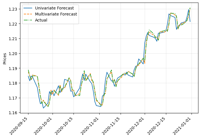
We can see that both results are almost the same, so multivariate forecasting isn’t justified in this case. Also, the results may seem good, but they are basically replicating the previous price with minimal change. In future articles we will see other Recurrent Neural Networks that may improve this result.