In the last article, we learned how to train a Machine Learning model like Linear Regression or XGBoost to forecast Time Series data. We had to reframe the dataframe as a supervised learning problem. You can read about this process here.
To explain the process we used Forex data, specifically the EUR/USD pair. We noticed that in the original dataset we also had other currency pairs such as GBP/USD, JPY/USD… What if we used this information to improve our model? There are two ways of achieving that:
- Adding them as exogenous variables: this is ideal if we just want to predict one currency pair, like EUR/USD
- Performing multivariate forecasting: this is the preferred option if we want to predict multiple pairs at once.
In this article, we will focus on the first one, a univariate model with exogenous variables.
Let’s begin by loading the data and preprocessing it as we did in the last article.
Data preparation
We need to:
- Import the required libraries
- Load the data
- Handle missing values
- Convert dates to datetime format and set it as index
- Reference all pairs to the same currency (USD in our case)
- Calculate the log returns to make our data stationary
# Import the required libraries
import pandas as pd
import numpy as np
from matplotlib import pyplot as plt

# Load the data
df = pd.read_csv('/kaggle/input/forex-data/data.csv')

# Handle missing values
df = df.ffill()

# Convert dates to datetime format and set it as index
df['Date'] = pd.to_datetime(df['Date'], format='%Y-%m-%d')
df = df.set_index(['Date'])

# Reference all pairs to the same currency (USD in our case)
for pair in df.columns:
    if (pair.split('/')[0] == 'USD') & (pair.split('/')[1] != 'USD'):
        df[f"{pair.split('/')[1]}/{pair.split('/')[0]}"] = 1 / df[pair]
        df = df.drop(columns=[pair])

# Calculate the log returns to make our data stationary
df_logret = np.log(df).diff()
df_logret.dropna(inplace=True)
For a step-by-step guide on how to do this consult my previous article.
This is how the last 30 days’ log returns look like:
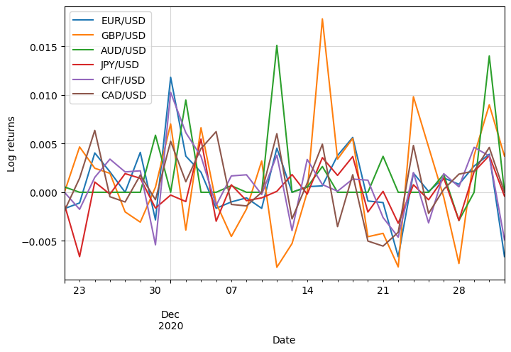
We can see that some of them increase on the same days, so they show signs of correlation.
Let’s calculate the correlation between pairs:
corr = df_logret.corr()
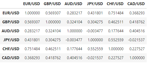
We can see that the Sterling Pound (GBP/USD) and the Swiss Franc (CHF/USD) show the largest levels of correlation, both above 0.50.
Univariate model with exogenous variables
To prevent adding noise to the model we will add only those highly correlated, in this case, GBP/USD and CHF/USD.
correlated_pairs = list(corr['EUR/USD'][1:][corr['EUR/USD'][1:] > 0.5].index)
We need to reframe our data to a supervised learning problem:
def reframe_to_supervised(df:pd.Series, window_size=7):
    # Initialize empty dataframe
    df_supervised = pd.DataFrame()

    # Define columns names
    X_columns = [f't-{window_size-i}' for i in range(window_size)]
    columns = X_columns + ['target']

    # Iterate
    for i in range(0, df.shape[0] - window_size):
        # Extract the last "window_size" observations and target
        # value and create an individual dataframe with this info
        df_supervised_i = pd.DataFrame([df.values[i:i+window_size+1]],
                                      columns=columns,
                                      index=[df.index[i+window_size]])

        # Add to the final dataframe
        df_supervised = pd.concat((df_supervised, df_supervised_i),
                                   axis=0)

    return df_supervised
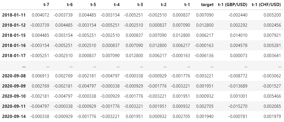
Using this function, let’s use a window of a week for the EUR/USD returns and a day for the other currencies:
# Features for the main currency pair
df_supervised = reframe_to_supervised(df_logret['EUR/USD'], window_size=7)

# Features for the pairs as exogenous variables
for pair in correlated_pairs:
    df_supervised_x = reframe_to_supervised(df_logret[pair], window_size=1, target=False)
    df_supervised = pd.concat((df_supervised, df_supervised_x), axis=1).dropna()
And this is how it looks:
Next, we need to split the dataframe into training and testing sets:
# Define the proportion of samples that will be added to the training set
training_proportion = 0.90

# We can calculate how many samples correspond to that proportion
n_obs = df_supervised.shape[0]
n_train = int(n_obs * training_proportion)

# Split dataframe in that proportion
df_train = df_supervised.iloc[:n_train]
df_test = df_supervised.iloc[n_train:]
We also need to split the features from the target:
X_train = df_train.drop(columns=['target'])
y_train = df_train['target']

X_test = df_test.drop(columns=['target'])
y_test = df_test['target']
Time to train the model!
import xgboost as xgb

# Convert the datasets into DMatrix
dtrain = xgb.DMatrix(X_train, label=y_train)
dtest = xgb.DMatrix(X_test)

# Set XGBoost parameters
param = {
    'max_depth': 3,
    'eta': 0.3,
    'objective': 'reg:squarederror'
}

# Number of boosting rounds
num_round = 100

# Train the model
bst = xgb.train(param, dtrain, num_round)

# Predict the target for the test set
y_pred = bst.predict(dtest)

# Calculate and print the RMSE
rmse = mean_squared_error(y_test, y_pred, squared=False)
print(f"RMSE: {rmse}")
RMSE: 0.003591956270337673
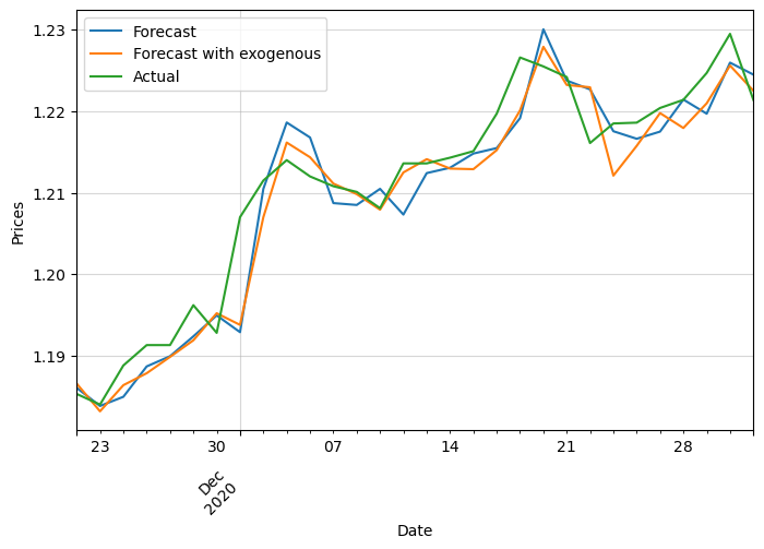
Finally, this is the result (compared to the case without exogenous variables):
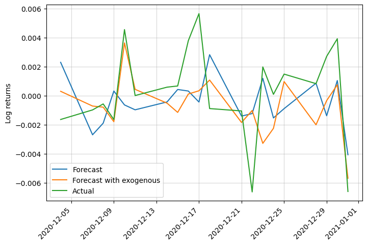
We can see that it performs slightly better, especially by capturing abrupt changes in trend. It went from a RMSE of 0.0036 to 0.0035.
Let’s check how the prices look after inverting the log returns transformation (check here if you want to see how to do it):
Univariate with additional exogenous variables
Similarly, we can add additional variables like details about the date, average of prices during the last week, or even technical indicators used in Forex trading.
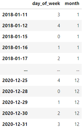
Temporal data
The features with more potential to be relevant to our model are the day of the week, especially if it is a weekend or not, and the month of the year.
# Calculate the day of the week
list_day = df_supervised.index.dayofweek
df_day = pd.DataFrame(list_day, columns=['day_of_week'], index=df_supervised.index)

# Calculate the month of the year
list_month = df_supervised.index.month
df_month = pd.DataFrame(list_month, columns=['month'], index=df_supervised.index)

# Merge it together
df_temp = pd.concat((df_day, df_month), axis=1)
This is what the additional temporal features look like:
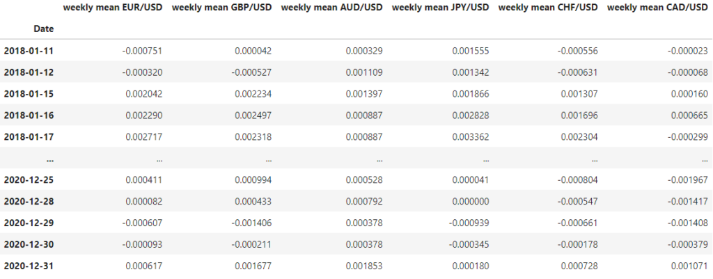
Average returns
We could also add some information about the average return during the previous week.
df_logret_mean = df_logret.shift(1).rolling(7).mean().dropna()
df_logret_mean.columns = ['weekly mean ' + pair for pair in df_logret_mean.columns]
The resulting features are:
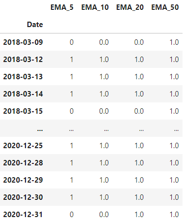
Exponential Moving Average
One of the most common technical indicators is the Exponential Moving Averages (EMA) of 5, 10, 20 and 50 days.
Let’s simply calculate them and check if the price is above (1) or below (0) this value.
First, we need to define the function to calculate the EMA and check the price:
def EMA(df:pd.Series, period:int, alpha=None):
    """
    Calculate Exponential Moving Average (EMA) for a list of prices

    :param prices: List of prices
    :param period: Period for which EMA needs to be calculated
    :param alpha: Smoothing factor (if None, then it's calculated as 2 / (period + 1))
    :return: List of EMA values
    """
    prices = df.values.flatten()

    if alpha is None:
        alpha = 2 / (period + 1)

    # Start with an SMA value for the first point
    ema_values = [sum(prices[:period]) / period]

    for price in prices[period:]:
        ema_values.append((1 - alpha) * ema_values[-1] + alpha * price)

    ema = [None] * (period - 1) + ema_values

    df_ema = pd.DataFrame(ema, index=df.index, columns=[f'EMA_{period}']).dropna()

    df_ema_indicator = df.loc[df_ema.index] > df_ema.iloc[:,0]
    df_ema_indicator = df_ema_indicator.to_frame(name=f'EMA_{period}')
    return df_ema_indicator.astype(int)
Finally, we apply it to the main pair (EUR/USD):
df_ema = pd.DataFrame()
for n_days in [5, 10, 20, 50]:
    df_ema_n = EMA(df['EUR/USD'], n_days)
    df_ema = pd.concat((df_ema, df_ema_n), axis=1)

# Drop missing values
df_ema.dropna(inplace=True)
And it looks like this:
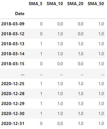
Simple Moving Average
We can do the same with the Simple Moving Average or SMA:
def SMA(df:pd.Series, period:int):
    """
    Calculate Simple Moving Average (SMA) for a list of prices

    :param prices: List of prices
    :param period: Period for which SMA needs to be calculated
    :return: List of SMA values
    """
    prices = df.values.flatten()

    sma_values = []
    for i in range(len(prices)):
        if i+1 < period:
            sma_values.append(None)
        else:
            sma_values.append(sum(prices[i+1-period:i+1]) / period)


    df_sma = pd.DataFrame(sma_values, index=df.index, columns=[f'SMA_{period}']).dropna()

    df_sma_indicator = df.loc[df_sma.index] > df_sma.iloc[:,0]
    df_sma_indicator = df_sma_indicator.to_frame(name=f'SMA_{period}')

    return df_sma_indicator.astype(int)
We apply it to the EUR/USD pair as follows:
df_sma = pd.DataFrame()
for n_days in [5, 10, 20, 50]:
    df_sma_n = SMA(df['EUR/USD'], n_days)
    df_sma = pd.concat((df_sma, df_sma_n), axis=1)

# Drop missing values
df_sma.dropna(inplace=True)
The resulting features are:
Merge all exogenous features
The last step is merging all features together and retraining the model:
df_supervised_exo = pd.concat((df_temp, df_ema, df_sma, df_logret_mean, df_supervised), axis=1)
df_supervised_exo.dropna(inplace=True)
Results
You can find below how the RMSE changed from our initial model to the latest one:
| Model | RMSE |
|---|---|
| Univariate | 0.00361 |
| Univariate with other pairs returns | 0.00359 |
| Univariate with exogenous variables | 0.00291 |
We can also check the log returns and price plots:
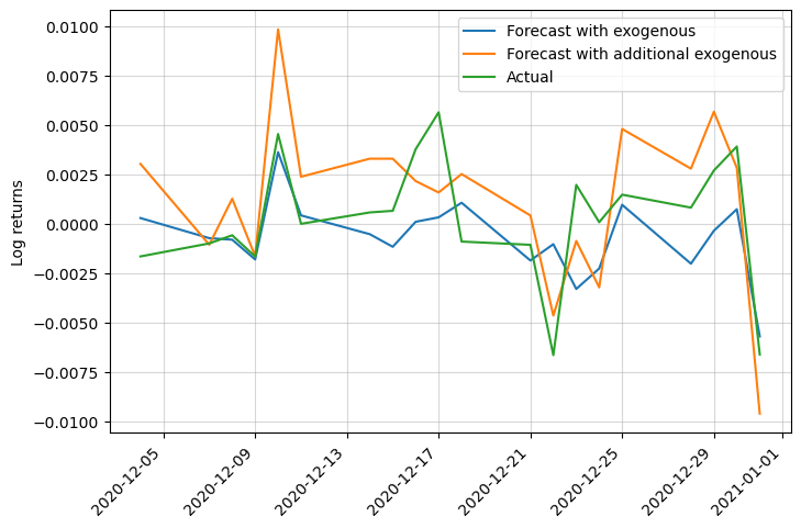
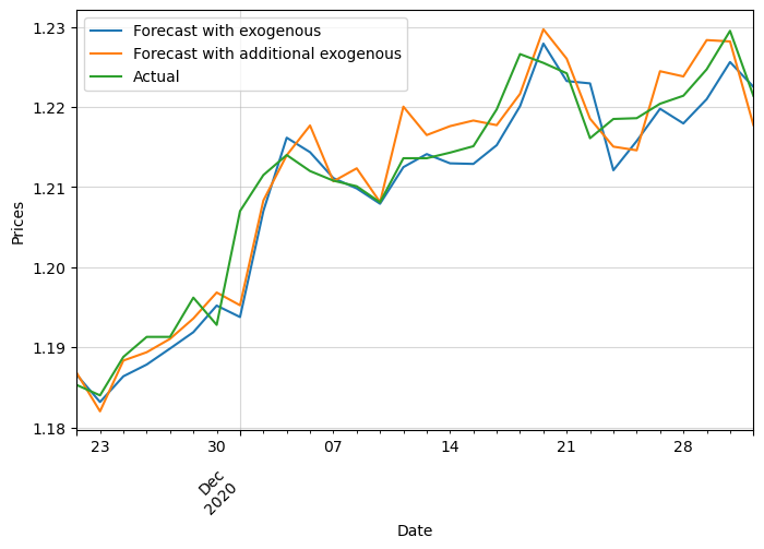
This was just an example of possible additional exogenous variables that you could add to your data. By adding more complex and meaningful features you could improve the performance of your model. Domain knowledge is key to achieving great models!
This exercise served you to learn how to train a Machine Learning model like XGBoost to do univariate Time Series forecasting. But what if you are interested in Multivariate forecasting, i.e., forecasting multiple variables at once? In our case, it would be forecasting EUR/USD, GBP/USD… with a unique model. We will see in the next article!


0 Comments