Clean your Time Series data I: Missing values and detrending

Time series data is a sequence of observations recorded at regular time intervals and is commonly used in various fields such as finance, economics, and engineering. However, time series data can often contain noise, outliers, missing values, and other anomalies that can affect the analysis and interpretation of the data. Hence, cleaning the data is an important step in the time series analysis process.

This article will provide a comprehensive overview of the steps involved in cleaning time series data. These steps, in the logical order in which they would normally be performed, are:

1. Handle missing values
2. Remove trend
3. Remove seasonality
4. Check for stationarity and make it stationary if necessary
5. Normalize the data
6. Remove outliers
7. Smooth the data

The article will also provide a general guideline for cleaning time series data and highlight the importance of using an appropriate approach for cleaning time series data. Please note that depending on your data, you will need to skip some steps or add modify or add other ones.

First steps

We will use a dataset from Kaggle that gathers the values of the monthly beer production in Australia from 1956 until 1995.

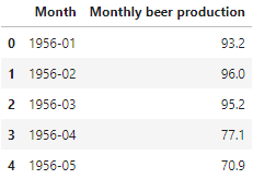
The first step after importing the data is inspecting it. We can start by checking the head (top 5 rows of data) of the dataset.

# Import required libraries
import pandas as pd
import numpy as np

# Read dataset file
df = pd.read_csv("/monthly-beer-production-in-austr.csv")

# Check data types
print(df.dtypes)

# Show the top five rows of the dataset
df.head()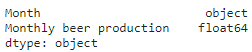

We notice two things:

• The date doesn’t have the right data type, it needs to be datetime.
• The index is not the date of the dataframe, and this is an important requirement when we are dealing with time series data.

So the next step would be to convert the date to datetime and set it as the index.

# Convert the month column to datetime
df['Month'] = pd.to_datetime(df['Month'], format='%Y-%m')

# Set the date as the index
df = df.set_index('Month')

# Convert the dataframe to series
df_beer = df['Monthly beer production']

Once this is done we can plot it:

# Import required libraries
import matplotlib.pyplot as plt

# Plot data
df_beer.plot(figsize=(14,6))
plt.xlabel('Date')
plt.ylabel('Monthly beer production')
plt.grid()
plt.show()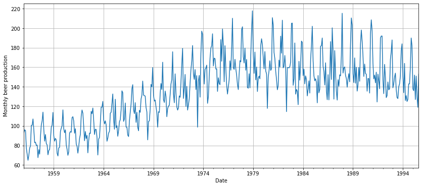

Let’s try to summarize the main concerns of the data just by having a quick look at the previous plot:

• It is non-stationary
• There seems to be a seasonal component
• There is a trend and an increasing variance
• It looks like there are some outliers

These are some of the issues we will need to address in the data-cleaning process.

Data cleaning

Handle missing values

We need to check whether we have missing values or not.

# Check for missing values
df.isna().sum()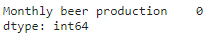

We are lucky this time, there are no missing values.

If we had, we could handle it by methods such as:

1. Imputation: these methods fill in the missing values with estimated values. Some popular imputation methods include constant value imputation, mean, median or mode imputation, and forward-fill or backward-fill.
2. Interpolation: these methods use mathematical functions to estimate missing values based on the values of the surrounding observations. The most popular ones are linear interpolation, polynomial interpolation, and spline interpolation.
3. Predictive Modeling: Predictive modelling methods use statistical or machine learning algorithms to build a model to predict missing values based on the values of other variables. Some popular predictive modeling methods include K-Nearest Neighbors, regression, decision trees, random forests, and neural networks.

It is important to choose an appropriate method for handling missing values based on the specific characteristics and requirements of the data. In some cases, a combination of methods may be necessary to obtain the best results. We show below how we would get rid of the missing values using some of the previously described methods:

# Imputation of constant value
df_beer = df_beer.fillna(0)

# Mean imputation
df_beer = df_beer.fillna(df_beer.mean())

# Backward-fill imputation (or last observation carried forward)
df_beer = df_beer.bfill()

# Linear interpolation
df_beer = df_beer.interpolate(method='linear')

But, as mentioned before, this is not necessary with the current data.

Remove trend

The majority of models, such as ARIMA, require stationary data. Stationarity is achieved when data has a constant mean, variance, and covariance.

The first step to achieving that is to remove the trend. The trend can be removed using different methods. Check below the most common ones:

1. Differencing: subtracting the observations from a previous time period to stabilize the mean of the series over time.
2. Decomposition: breaking down the time series into its trend, seasonal, and residual components and removing the trend component.
3. Moving averages: calculating the average of the observations over a fixed number of time periods and subtracting it from each observation.
4. Polynomial fitting: fitting a polynomial curve to the time series data and subtracting it from the original series to remove the trend.
5. Trend filters: using filters such as Hodrick-Prescott or Kalman filter to remove the trend component.
6. Log Transformations: taking the logarithm of the time series data to reduce the magnitude of the trend and stabilize the variance of the series.
7. Box-Cox Transformations: transforming the time series data using a power transformation to stabilize the variance and make the trend linear.

Depending on the specific requirements and characteristics of the data one technique may be more suitable than other. In some cases, more than one method will be required.

For our example, we will show the first one, which is one of the most frequently used. After we take the first difference of the data we need to remove the first row of our data. This is because we are not able to get the difference of the first element as there is no other value before. Therefore, it appears as NaN (Not a Number) and can just be dropped.

# Take the first difference of the data to remove the trend
df_beer = df_beer.diff()

# Drop the first NaN value coming from taking the difference 
df_beer = df_beer.dropna()

# Plot the data to see the outcome
df_beer.plot(figsize=(15,5))
plt.xlabel('Date')
plt.ylabel('Beer production increase rate')
plt.grid()
plt.show()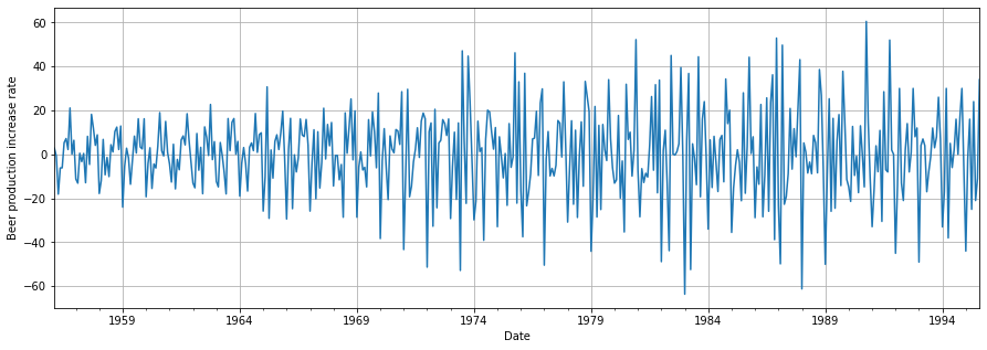

We observe that the mean is now approximately constant around zero. However, there is still another issue to sort out: the non-constant or increasing variance.

We could use some of the transformations seen before. however, we will use an intuitive approach instead. To address the continuously increasing variance over the years, we could enforce a consistent variance for each year. Let’s see how we can achieve this in Python.

# Calculate each year's variance (equivalent to standard deviation)
annual_variance = df_beer.groupby(df_beer.index.year).std()
mapped_annual_variance = df_beer.index.map(
    lambda x: annual_variance.loc[x.year])

# Standardize each year's variance
df_beer = df_beer / mapped_annual_variance

# Plot outcome
df_beer.plot(figsize=(15,5))
plt.xlabel('Date')
plt.ylabel('Standardized beer production rate')
plt.grid()
plt.show()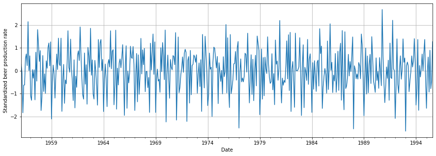

We can finally see how our data has a constant variance and mean. We are now a step closer to achieving stationarity!

See all the parts of the data cleaning series:

1. Missing values and detrending
2. Remove seasonality and normalize data
3. Outliers removal
4. Data Smoothing

You can access the notebook in our repository:

GitHub – MLPills/missing-values-and-detrending: A Jupyter Notebook that covers the basics of dealing with missing values as well as how to remove the trend from out time series dataset

A Jupyter Notebook that covers the basics of dealing with missing values as well as how to remove the trend from out time series dataset – GitHub – MLPills/missing-values-and-detrending: A Jupyter Notebook that covers the basics of dealing with missing values as well as how to remove the trend from out time series dataset

github.com

To run it right now click on the icon below:

We will see in the next article how we can check and remove the seasonality!